Adding an ordinal\r\nindicator – st, nd, rd, and th – uses a suffix to denote the value’s\r\nposition within a series. For example, 1 becomes 1st, 2 becomes 2nd, 3 becomes\r\n3rd, and so on. In Excel, you can use a complex formula to create a new string or\r\nyou can apply several conditional formatting rules to display the indicator\r\nwith the value.
\r\n\r\n
Excel 2003 users must use the formula solution. If you want\r\nto apply the conditional formatting technique, you must have Excel 2007 or\r\nlater.
\r\n\r\n
\r\n\r\n
Knowing the rules and their precedence is imperative. Trying\r\nto apply ordinals without knowing the following rules will just make you sad:
\r\n\r\n
\r\n
\r\n
\r\n
\r\n
\r\n
\r\n\r\n
Getting the rules applied in the correct order is the key.\r\nThe values 11, 12, and 13 certainly throw a monkey wrench into the works, but\r\nExcel can handle it.
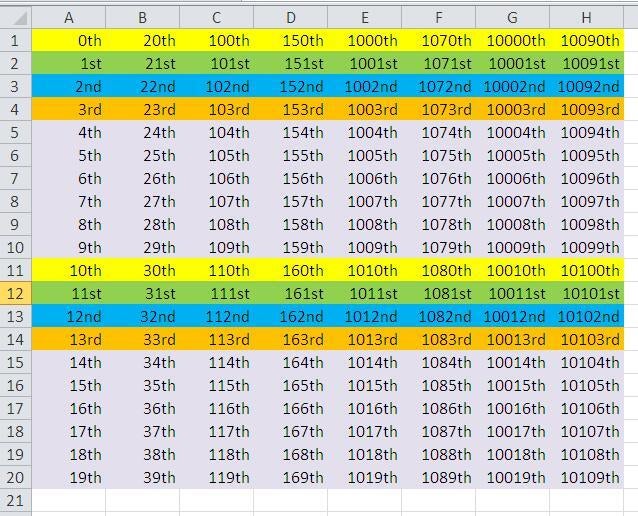
In the figure below, I’ve used a formula to combine a value\r\nand its appropriate ordinal indicator:
\r\n\r\n
=value&IF(AND(MOD(ABS(value),100)>10,MOD(ABS(value),100)<14),"th",CHOOSE(MOD(ABS(value),10)+1,"th","st","nd","rd","th","th","th","th","th","th"))
\r\n\r\n
This formula has been in use for a long time. If you try a\r\nshorter version, be sure to check the results for values ending with 11, 12,\r\nand 13 carefully. Most importantly, this formula returns a string, not a value;\r\nyou can’t refer to the results of the formula in mathematical equations.
\r\n\r\n
Although long, the formula is simple. The first part of the\r\nformula accommodates values ending with 11, 12, and 13. The second part of the\r\nformula uses CHOOSE() to handle the rest. I suppose you could simplify both\r\ncomponents, but I’ve never tried. This works, and I can’t justify the time it\r\nwould take to rethink it. It works with positive and negative integers,\r\nignoring decimal components.
\r\n\r\nCredit: Image by Susan Harkins for TechRepublic
\r\n\r\n
You can also use a conditional format. This method displays\r\nthe indicator with the actual value rather than creating a new string. The\r\noriginal value remains a numeric value. You only change the way Excel displays\r\nthat value.
\r\n\r\n
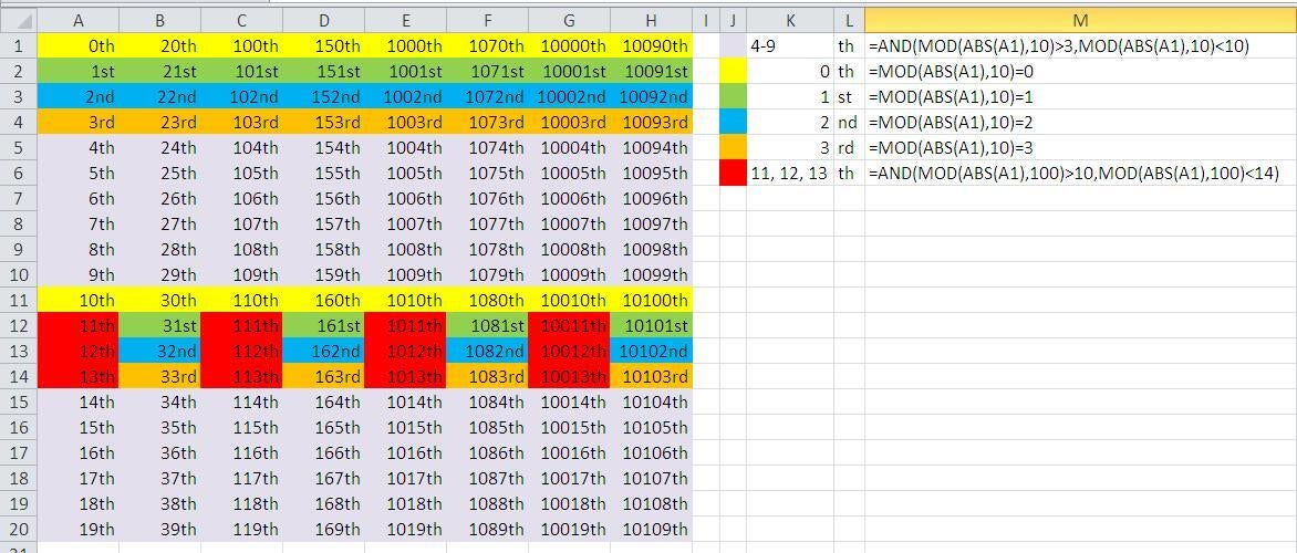
You’ll need six formulas instead of one; use the formulas\r\nlisted in Table A.
\r\n\r\n
\r\n\r\n
\r\n\r\n\r\n\r\n\r\n\r\n\r\n\r\n\r\n\r\n\r\n\r\n\r\n\r\n\r\n\r\n\r\n\r\n\r\n\r\n\r\n\r\n\r\n\r\n\r\n\r\n\r\n\r\n\r\n\r\n\r\n
| \r\n
\r\n |
\r\n
\r\n |
\r\n
\r\n |
| \r\n
\r\n |
\r\n
\r\n |
\r\n
\r\n |
| \r\n
\r\n |
\r\n
\r\n |
\r\n
\r\n |
| \r\n
\r\n |
\r\n
\r\n |
\r\n
\r\n |
| \r\n
\r\n |
\r\n
\r\n |
\r\n
\r\n |
| \r\n
\r\n |
\r\n
\r\n |
\r\n
\r\n |
\r\n\r\n
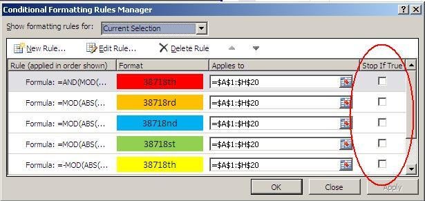
You must enter the\r\nabove rules in their listed order. There are other routes and other formulas,\r\nbut this route specifies each rule in ordinal precedence. If you use other\r\nrules, be sure to account for the application order, which can get messy – it\r\nisn’t impossible, but it is more\r\ndifficult to follow.
\r\n\r\n
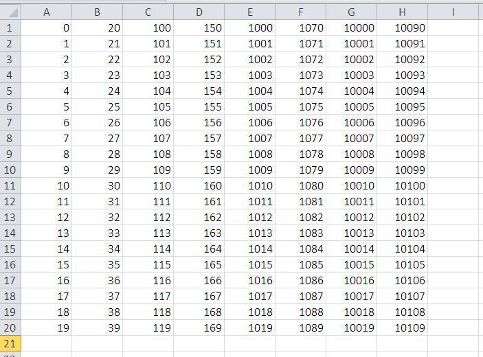
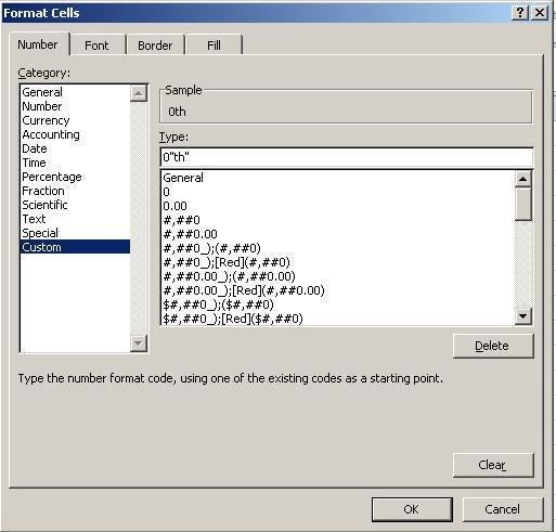
Now, let’s apply the first rule to the values shown below:
\r\n\r\n
\r\n
\r\n
\r\n
\r\n
\r\n
\r\n\r\n
=AND(MOD(ABS(A1),10)>3,MOD(ABS(A1),10)<10)
\r\n\r\nCredit: Image by Susan Harkins for TechRepublic

\r\n
\r\n
\r\n
\r\n
\r\n\r\n
You can skip that last step if you like. I’m also using\r\ncolor to highlight the formatted values. Doing so creates a nice visual trail\r\nto follow, but you probably won’t want to apply color to the values you format\r\nin your own sheets. Click the Fill tab, choose a color, and click OK.
\r\n\r\n
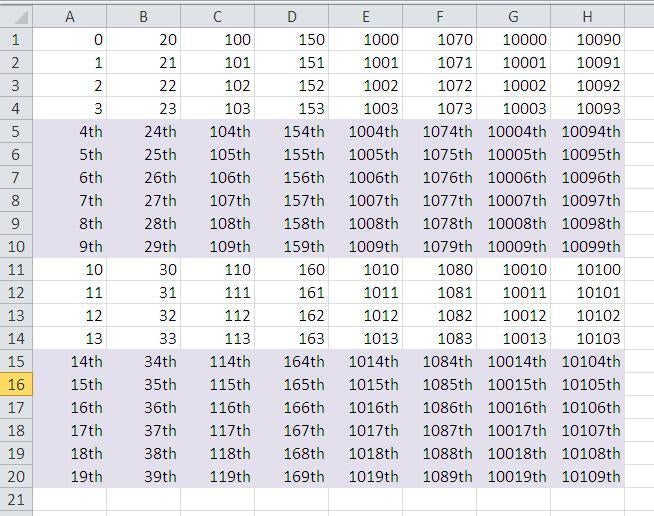
Click OK twice. This first rule adds th to values ending\r\nwith the digits 4 through 9.
\r\n\r\n
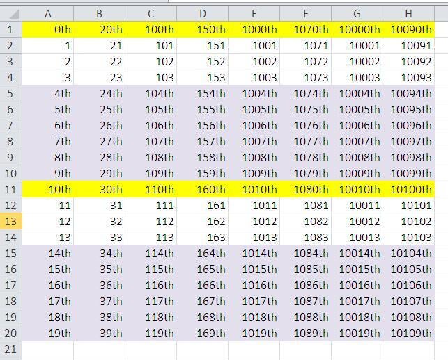
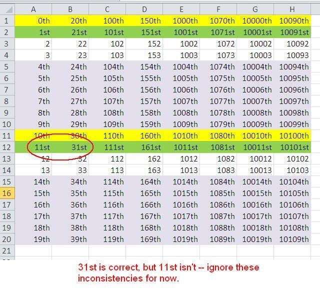
Repeat this process for the remaining rules, being careful\r\nto add them in the listed order. When you enter the rules for 1, 2, and 3,\r\nyou’ll notice that Excel also formats the values ending with 11, 12, and 13,\r\nwhich is incorrect. Don’t worry because the final rule for 11, 12, and 13 will\r\noverride the earlier rules where necessary.
\r\n\r\nCredit: Image by Susan Harkins for TechRepublic
Credit: Image by Susan Harkins for TechRepublic
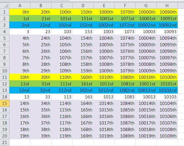
\r\n\r\nUsing conditional formats\r\nto apply ordinal indicators can be problematic. First, you must be careful to\r\nconsider precedence when entering the rules. My way isn’t the only way and it\r\nisn’t the most efficient, but it is easy to follow. Second, if you’re working\r\nwith other conditional formats, you must continue to consider precedence. You\r\ncan combine rules and use the Stop If True property appropriately when\r\ncombining this set of rules with others. Next month, I’ll show you how to add\r\nordinal indicators to dates.
\r\n\r\nCredit: Image by Susan Harkins for TechRepublic