DIY: Conditional formatting in LibreOffice Calc

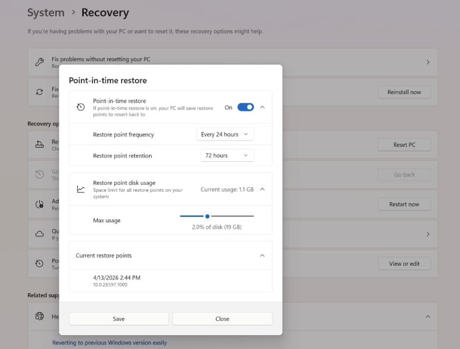
Sometimes you discover a feature that makes using a particular tool incredibly efficient. Conditional formatting is that feature in LibreOffice's spreadsheet application Calc.

What is conditional formatting?

Let's say you are about to create a huge spreadsheet, and certain cells must be formatted in a specific way based on other cells. For example, any cell with a number under a specific value must be formatted with a green background and over a specific value is formatted with a red background. Instead of going back and formatting each cell, conditional formatting will do this automatically.

In this tutorial, I walk through how to create this kind of formatting. We'll stick with my example:

• Value < 100 = Green
• Value > 100 = Red

The first step is to create the styles you want to use for the conditional formatting by following these steps in Calc:

1. Open the Styles And Formatting window from within Calc by going to Format | Styles And Formatting.
2. Make sure you're on Cell Formatting (upper left corner) and then right-click any blank area in the window and select New.
3. In the resulting window, give the style an appropriate name in the Organizer tab (Figure A).
4. Go to the Background tab and create the style appropriate for the value.
5. Click OK.

For our example, you would need to create two styles:

• One with a green background for the value under 100.
• One with a red background for the value over 100.

In the Conditional Formatting window, follow these steps:

1. In the first row of drop-downs, select Cell Value Is and Less Than.
2. In the text area, enter 100.
3. In the Cell Style drop-down, select the new style you created for the green value (in my case, I called it GreenValue).
4. Go to the second condition and create the second condition for the red value (greater than 100).
5. Click OK.

One number that wasn't addressed in the conditions is 100.

Conditional formatting doesn't just work with cell values; you can also use formulas for conditions, and you can mix and match. For example, you could have a condition that does the following:

If a formula is A * B and the result is equal to or greater than 100, the background is red and the font is bold. Set a second condition that if a formula is B * C and the result is equal to or greater than 100 the background is green and the font is italics.

You can get pretty creative with conditional formatting. Even though you are limited to only three conditions, you can do quite a lot to help get your spreadsheets formatted correctly and efficiently. You no longer have to go back, highlight cells, and manually format cells according to numerical number.