How to Extract a Substring in Excel Using FIND() and MID() Functions

Parsing data is a common task in Excel. For the most part, you’ll do so when you need to work with substrings rather than the whole source values. For instance, you might want to parse a store or customer identification number from a transaction string that includes all the information about a specific transaction.

Thanks to Excel’s string functions, parsing is easy, as long as the source values are consistent. String functions, such as MID() need to know where the substring you’re extracting begins and ends. When that information is unknown or inconsistent from one value to another, you’ll have to work a bit harder.

In this article, I’ll show you how to combine two string functions, MID() and FIND() to solve the problem of parsing structurally inconsistent data. I’m using Microsoft 365, but these functions are available in standalone versions.

Jump to:

• What are string functions?
• How to use the MID() function
• How to use the FIND() function
• How to combine MID() and FIND()

What are string functions?

MID() and FIND() are string functions. In Excel, string functions let you retrieve specific characters, also called a substring, from a source string. There are several string functions:

• LEFT(): Gets characters from the left side of the source string.
• RIGHT(): Gets characters from the right side of the source string.
• MID(): Gets characters from the middle of the source string.
• LEN(): Returns the number of characters in the source string.
• FIND(): Returns the position of a specific character within the source string.

By using these functions separately or by combining them, you can quickly return a substring from a source string.

How to use the MID() function

When extracting a substring — a smaller piece of the source string — from the middle of the source string, you might consider using MID(), which uses two arguments to retrieve characters from the middle of a string. It uses the form:

MID()(text, start_num, num_chars)

where text is the source string, start_num is the position of the first character you want to parse and num_chars is the total number of characters you want to parse.

Let’s look at a quick example using the sample data shown in Figure A.

Figure A

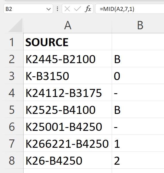
Specifically, let’s return the first character following the hyphen character from each source string in the dataset as follows:

1. In B2, enter the following function
   =MID(A2,7,1)
2. Copy it to the remaining cells in the dataset.

The argument, 7, begins the parse at the seventh character in A2 and 1 specifies that the function parses only one character, returning the letter B from the source string in A2.

If you copy the function to the remaining cells in the dataset, you’ll notice that it often fails. Our original task was to return the first character following the hyphen character. Unfortunately, the hyphen isn’t always in the seventh position — that position is inconsistent.

If the hyphen were positioned consistently, MID() would work. But what do you do when the substring you want to extract could start anywhere within the string? Here’s the trick: You use the FIND() function to return the position of the hyphen and then use those results as the MID() function’s second argument. So next, let’s learn how to use FIND().

SEE: 3 Ways to Suppress 0 in Excel.

How to use the FIND() function

Excel’s FIND() function parses a substring by finding the position of a specific character or string. This function uses the form

FIND(find_text, text, [start_num])

where find_text is the substring you’re looking for, text is the source string you’re searching and start_num specifies the character at which to begin the search. When omitted, the search always begins with the first character in text.

Now, let’s use FIND() to return the position of the hyphen character:

1. In C2, enter the function
   =FIND(“-“,A2)
2. Copy it to the remaining cells in the dataset (Figure B).

Figure B

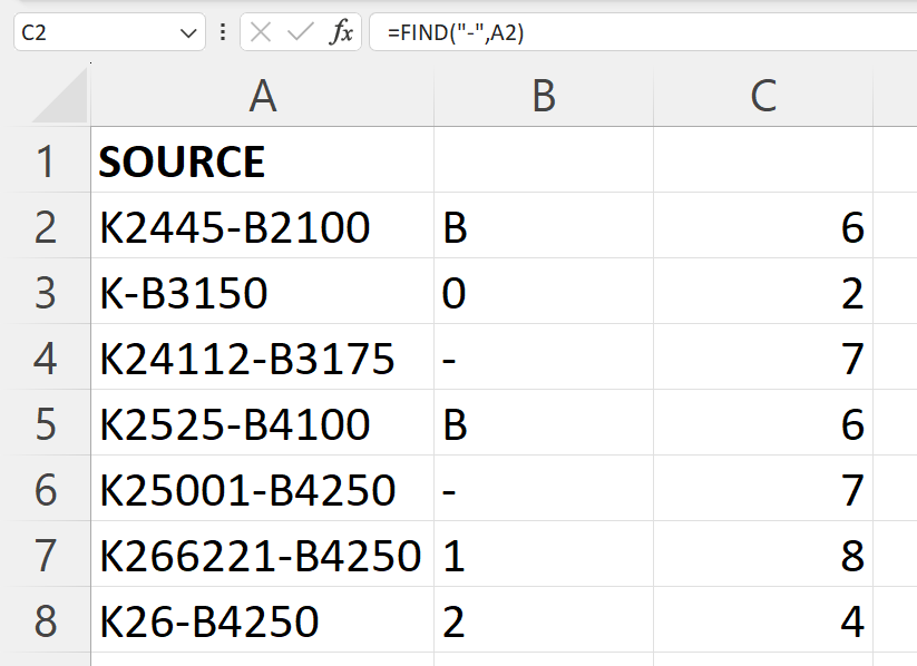
As you can see, FIND() returns a value, not a character. This value represents the position of the found character, in this case, the hyphen character.

SEE: How to parse data in Microsoft Excel.

How to combine MID() and FIND()

We know a couple of things at this point: MID() returns a substring from the middle of a source string and FIND() returns the position of a specific string within a source string. When the source data is inconsistent in structure but each value has a common character, you can combine the two functions to get the job done.

We’ve already used FIND() to return the position of the hyphen in each value. Now, let’s combine it with MID() to return the character that immediately follows the hyphen in each value, as follows:

1. In D2, enter the following function
   =MID(A2,FIND(“-“,A2)+1,1)
2. Copy it to the remaining cells in the dataset (Figure C).

Figure C

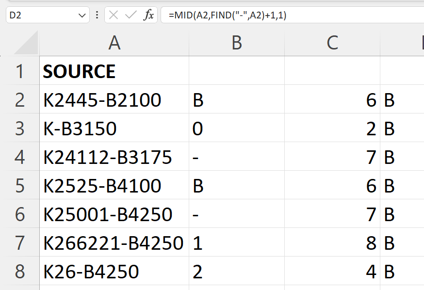
Now, let’s review how the combination works using the first value in the dataset, K2445-B2100:

=MID(A2,FIND("-",A2)+1,1)

=MID(K2445-B2100,FIND("-",K2445-B2100)+1,1)

=MID(K2445-B2100,(6+1),1)

=MID(K2445-B2100,(7),1)

=MID("B",1)

=B

The FIND() function returns 6, the position of the first hyphen in K2445-B2100. The MID() function then uses the value 6 (plus 1) to return B. We add the value 1 to move the extraction to the right by one character. We’re parsing the character to the right of the hyphen, not the hyphen.

Thanks to FIND(), the hyphen character can be anywhere within the source string and we can still find a character relative to it.