How to Suppress 0 in Excel in 3 Ways

If you want to hide or suppress zero values in a spreadsheet, Excel offers three easy ways to get these results. In this Excel tutorial, I’ll show you how to implement a setting, a format or a function solution to hide or suppress zeros.

I’m using Microsoft 365 on a Windows 11 64-bit system, but you can use also use alternative versions. To follow along, you can work with your own data or download the demonstration .xlxs file. Excel for the web will display the results correctly; however, the last method is the only one that you can implement in the browser.

How to suppress 0s in an entire Excel sheet

The easiest method to suppress zeros in Excel is a simple setting with an all-or-nothing result, which is both a pro and a con, depending on your needs. To suppress zeros at the sheet level, do the following:

1. Click the File tab, choose Options in the left pane and then click Advanced in the left pane.

2. In the Display options for this worksheet section, uncheck Show a zero in cells that have zero value (Figure A).

Figure A

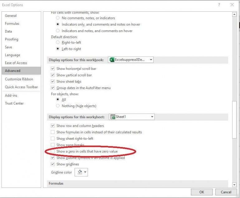
Uncheck this option to suppress zero values.

3. Click OK to close the dialog.

Figure B shows the results of unchecking this option to the right; for comparison, on the left you can see where zeros, expressions that evaluate to zero and blanks were. The blanks remain blank, and the cells containing zero values are blank. In addition, the formulas in D5 and D7 that return zero are blank. However, the currency format is still visible.

Figure B

SEE: Learn how to enter leading zeros in Excel.

There are no visible zero values. They’re still there, but  the entire Excel sheet is suppressing their display. If you like, try to enter zero or an expression that returns zero in an empty cell. You can enter it and see it in the Formula bar, but you can’t see it in the cell. Although you can’t see the zeros, Excel still evaluates the contents as zero when referenced.

If this setting is overkill, you can use a custom format. If you’re working with the demonstration file to follow along, be sure to reset this option before continuing or use the data in the Format sheet.

SEE: Check out these Excel tips every user should master.

How to use a format to suppress 0s in a range in Excel

Instead of using the far-reaching sheet-level option, you can limit the Excel cells that suppress zero by applying a custom format to a range of cells. As a result, you control which cells will  suppress zeros. You get more control with this method, but it does usurp your formatting capabilities and might require a bit of thought — you’ll see why this matters in a minute.

Review syntax

Before continuing, we need to review a custom format’s structure, or syntax:

positive; negative; zero; text

The simplest custom format that will suppress zero is:

0;0;;@

The zeros in the positive and negative positions are placeholders and will display any positive or negative value. Leaving the third component — the zero component — empty is what suppresses zeros. To display zeros as 0, you’d enter 0. The @ is a text placeholder, similar to the 0 placeholder.

SEE: Here’s how to create a drop-down list in Excel.

Apply custom formatting

Now, let’s apply this custom format and see what happens:

1. Select the range you want to format. In this case, that’s B3:D7.
2. Click the Number group’s dialog launcher button on the Home tab.
3. In the Category list, click Custom at the bottom.
4. Enter 0;0;;@ in the Type control (Figure C).

Figure C

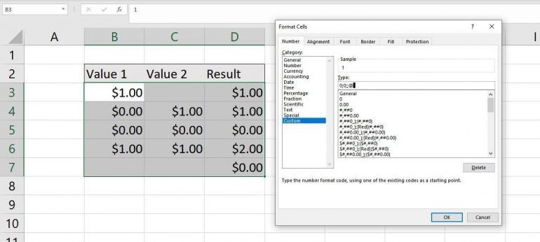
5. Click OK to close the dialog.

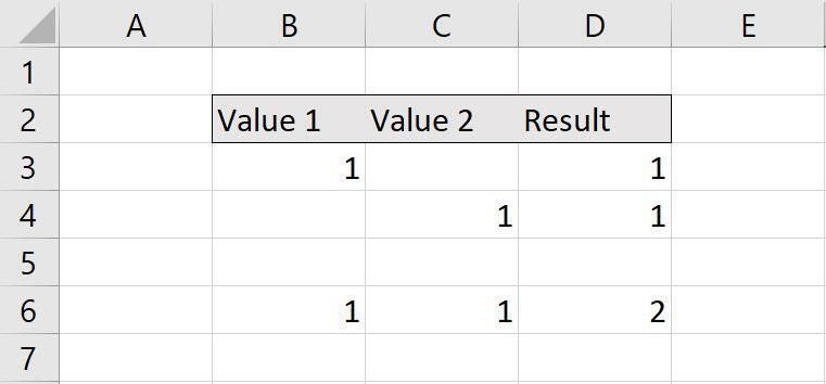
At first, it looks like it worked fine, but if you compare the formatted results in Figure D to the original data in Figure B, you’ll see we’ve lost the currency symbol and the decimal places.

Figure D

SEE: Learn how to parse time values in Microsoft Excel.

Modify the custom formatting

We can easily modify the custom format so it accommodates our needs. Specifically, retry the $0.00;$0.00;;@ format. In Figure E, you can see that the second format maintains the currency symbol and decimal places.

Figure E

This custom format is more comprehensive than the first one we tried.

If a custom format won’t work for your needs, you might want to use a formula. Be sure to reset the custom format before you continue to the next section or use the IF() sheet.

SEE: Follow along to learn how to parse data in Microsoft Excel.

How to use a formula to suppress 0 in a cell in Excel

When using an expression that might return a zero, you can wrap that expression in an IF() function to suppress a zero result. Generally you won’t want to do this, but to be comprehensively prepared, you’ll want to know how to do this.

SEE: Discover how to apply Insights in Excel.

Our simple expression in column D is =B3+C3, and D5 and D7 return zero. Select cell D3 and enter the expression:

=IF(B3+C3=0,””,B3+C3)

Then, copy it to D4:D7. Figure F shows the results; D5 and D7 are now blank.

Figure F

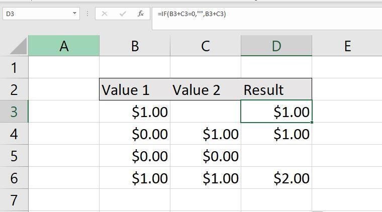
You can hide zeros using an IF() function.

The IF() function evaluates the expression that sums the two values and returns an empty string (“”) when the result is zero; if it isn’t zero, the IF() returns an empty string, as indicated by the “” string. The big difference between this solution and the first two is that you’ll use this only with expressions, not values. In addition, you can control which expressions return the empty string instead of zero.