


Summarizing data is one of Microsoft Excel’s main functions. The good news is that a lot of number crunching can be done on the fly and without any specialized knowledge. You might need a quick sales total during a meeting, or perhaps, you’re trying to put together a quick report before a meeting. Fortunately, Excel has a few quick summarizing features that seem almost magical and will help you look good when time is short.
I’m using Microsoft Excel on Office 365 (desktop) on a Windows 11 64-bit system, but these tips will work in older versions and in the browser edition.
Jump to:
- How to use the status bar to summarize Excel data
- How to use AutoSum to summarize Excel data
- How to filter a table in Excel
- Easy summarizing
How to use the status bar to summarize Excel data
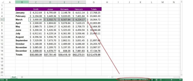
The status bar provides instant gratification when summarizing — all you have to do is select the values. Figure A shows the March values selected. The status bar responds by displaying the average, count and sum of the selected values.
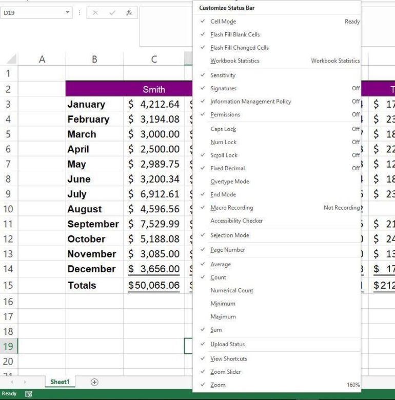
That’s not all. You can customize the status bar to display exactly the information you need. Simply right-click and check the appropriate options (Figure B).
SEE: Explore these Excel tips and tricks for beginners and pros.
How to use AutoSum to summarize Excel data
Using the data shown in Figure A, let’s move on to the AutoSum feature:
- Click G3.
- Click AutoSum in the Editing group on the Home tab. Before pressing Enter a second time, you can see that AutoSum inserted a SUM() function that evaluates all of the contiguous values to the left (Figure C). The feature knows the label in B3 isn’t a value, so it stops at C3.

- Press Enter a second time to commit the default SUM() function.
Note that the AutoSum option has a dropdown that offers several other functions; SUM() is the default. If you want to use a different function, simply select a different option and continue.
SEE: How to Extract Delimited Data Using Excel Power Query
How to filter a table in Excel
Excel allows you to apply a summarizing filter by clicking Filter in the Sort & Filter group on the Data tab. This displays dropdowns in each header cell, which you can click to explore filtering options.
Instead of pursuing filtering options right now, let’s convert this ordinary data range into a Table object. You must format the data range as a Table object in order to add a summarizing row. The setup takes a few easy steps to implement:
- Click anywhere inside the data range.
- Click the Insert tab.
- Click Table in the Tables group.
- In the resulting dialog, confirm whether your data range has headers (ours does), and click OK.
The Table object has a neat feature: a totaling row. When combined with the built-in filtering feature, it evaluates only the filtered set. To illustrate, do the following:
- Click anywhere inside the Table.
- Click the contextual Table Design tab.
- In the Table Style Options group, check the Total Row option.
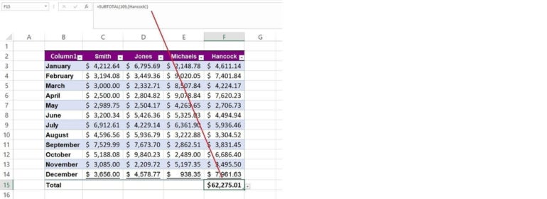
Figure D shows the results of a SUBTOTAL() function, which is a powerful and flexible function you’ll want to explore further. Similar to AutoSum, you can change the function’s purpose. In addition, you can add a function to each column in the Table.
SEE: How to use TODAY() to highlight fast-approaching dates in Excel.
Easy summarizing
You can’t always use summarized results in further calculations, but you won’t always need to. Sometimes, you only need a quick look at what’s going on, and that’s when these techniques will come in handy and really help you shine.