
Microsoft Excel’s Subtotal feature calculates subtotals and a grand total for columnar data, but that’s not all. This Excel feature supports 11 calculating processes: sum, count, average, maximum, minimum, product, count number and more. The good news is that Excel’s Subtotal feature requires very little setup–in less than a minute, you can render a rather complex problem into results. Unfortunately, there’s scant little formatting. In this Excel tutorial, I’ll show you how to run subtotals on a simple data set and then quickly apply formatting that will make those totals really stand out.
SEE: Software Installation Policy (TechRepublic)
If you’re not familiar with Excel’s Subtotal feature, read How to use Excel’s Subtotal feature, 10+ tips for working with Excel’s Subtotal feature and How to use a conditional format to highlight subtotal rows in Excel. However, you should be able to follow the steps in this article without prior knowledge of the Excel feature.
I’m using Microsoft 365 on a Windows 10 64-bit system, but you can use an earlier version. I recommend that you hold off on upgrading to Windows 11 until all the kinks are worked out. This Excel feature is available only in ribbon versions (.xlsx). For your convenience, you can download the demonstration .xlsx file.
Disclaimers for when you use Excel’s Subtotal feature
Consistency is the word of the day when using Excel’s Subtotal feature. The columns you use to generate the subtotals must contains consistent data. For instance, if a department column contains inconsistent values such as H&R and HR, this feature will not return the correct results. Instead of evaluating H&R and HR as one group, it will evaluate them as two and if you don’t catch it, you might pass on erroneous information.
The next important issue is you must sort the data before applying the Subtotal feature. If you’re subtotaling billable hours for each department, you must sort by the departments first. That way, the groups are already in place before you turn to Subtotal.
A simple run of Excel’s Subtotal feature
The data in Figure A is a data range, and not a Table object. That’s because, for now, you can not run the Subtotal feature on data in a Table object. Now, let’s apply Subtotal to return a subtotal for the invoice amounts for each vendor.
Figure A
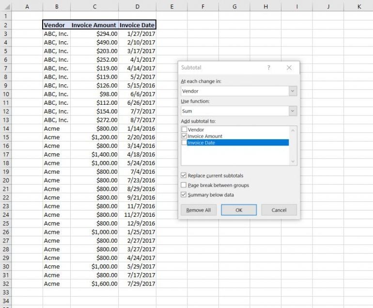
First, sort the data range if necessary, by the vendor. As you can see, ours is already grouped by vendor. If you’re applying this to your own work, you might want to sort now. With the data sorted by the vendor group—in this case, that’s the vendor—you’re ready to apply the Subtotal feature:
Click any cell inside the data range and click the Data tab.
In the Outline group (to the far right) click Subtotal.
The resulting dialog tries to anticipate your needs. It may or may not be correct. From the At Each Change In dropdown, choose Vendor—that’s the group. From the Use Function dropdown, choose Sum. There are many other options to choose from though. In the Add Subtotal to list, check only Invoice Amount (Figure A). We only want to sum the invoice amounts for each vendor. To commit, click OK to see the results in Figure B.
Figure B
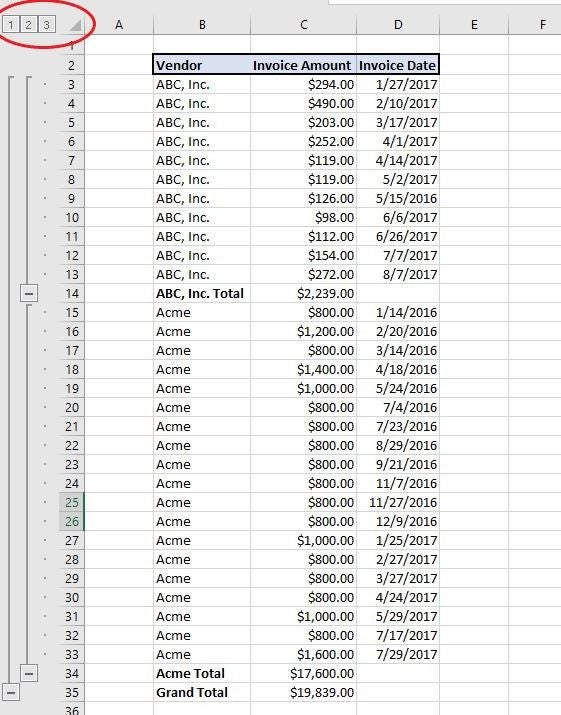
As you can see, the invoice subtotals for each vendor don’t stand out. Fortunately, a few quick formatting tricks will make them stand out, loud and clear.
How to format subtotals in Excel
What this list needs is some formatting to make those vendor subtotals stand out. At the left, you can see the three grouping levels: 1, 2 and 3. To show only the subtotals, click button 2, which will display three rows: two subtotal vendor rows and one grand total row.
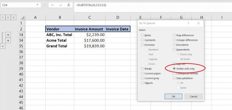
At this point, any formatting you add to the subtotaling rows will be applied to those rows and the hidden rows, and that’s not what you want. Fortunately, we can use the Visible Cells Only option to format only the three rows visible once you click button 2. If you skip this step, Excel will select all the visible cells in the worksheet.
To apply this option, do the following:
Select the values in column C—you want to format the subtotal invoice values (C14:C35, which includes the hidden rows).
Click the Home tab, click Find & Select in the Editing group, and then click Go To in the resulting dropdown.
In the resulting dialog, click the Special button (bottom-left).
In the next dialog, click the Visible Cells Only option (Figure C) and click OK.
Figure C
With the current selection, click Bold in the Font group on the Home tab.
Select the two subtotals and repeat step 2 through 4 to choose only the visible cells.
Then, click the Font group’s Dialog Launcher to access more options.
In the resulting dialog, click the Font tab and choose Single Accounting from the Underline dropdown and click OK. Doing so display a single underline in the subtotal cells.
Select the grand total value and apply a Double Account underline in the same way (Figure D).
Figure D
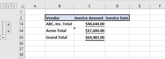
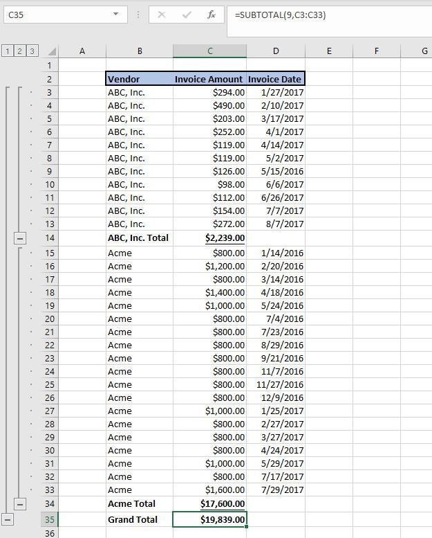
If you click button 3, you can see the new formats, as shown in Figure E. If some of the original values are bold or underlined, press Ctrl + Z and repeat the above instructions, remembering to select the Visible Cells Only option.
Figure E
You could stop here, but you might want that subtotal and grand total to stand out just a bit more by moving them to the right into a column of their own.
If you clicked button 3, click button 2 to collapse the data and do the following:
Select only the visible cells as you did before, remembering to select C13:C35 first. Remember, there are hidden rows in that range. Don’t skip this step!
To shift these three values to the right, click the Home tab.
In the Cells group, click the Insert option and choose Insert Cells.
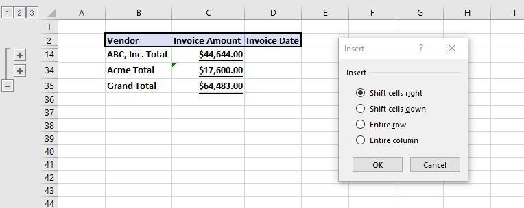
The default values, shown in Figure F is the right option, so click OK.
Figure F
Repeat the steps again but the values are now in column D (D13:D35).
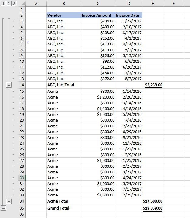
To see the formatted results, click button 3. The subtotals and grand total values really stand out now, as shown in Figure G. You could continue to apply more formatting, but these seem to get the job done for this particular subtotal set.
Figure G
The only cons to the Excel Subtotal
The formatting applied is temporary. It’s great for a quick print out, but it doesn’t stick. If you remove the subtotals and then reapply the feature, you will have to reapply the formatting. If you’d like something more permanent, read How to use a conditional format to highlight subtotal rows in Excel.
Before doing anything with the subtotals, you must remember to apply the Visible Cells Only option. If you forget, Excel will apply the format to all of the data cells as well. It can be frustrating, but remember, Ctrl+Z will undo the mistakes quickly so you can try again.


