How to use the new TEXTAFTER() and TEXTBEFORE() functions in Microsoft Excel

A common task is to parse or find characters within a delimited string in Microsoft Excel. Fortunately, Excel has several string functions to help, but the resulting expressions are complex. Power Query doesn’t require complicated expressions, and Flash Fill is great at finding patterns, but the release of Excel’s two new text functions will simplify things even further.

In this tutorial, we’ll briefly review two new text functions: TEXTAFTER() and TEXTBEFORE(). We’ll focus on TEXTAFTER(), but everything you learn applies to TEXTBEFORE() other than the direction of the extracted characters.

SEE: Google Workspace vs. Microsoft 365: A side-by-side analysis w/checklist (TechRepublic Premium)

I’m using Microsoft 365 on a Windows 10 64-bit system. Microsoft rolled these functions out in September, so they should be available to all Microsoft 365 subscribers, which includes Excel for the web.

You can download the Microsoft Excel demo file for this tutorial.

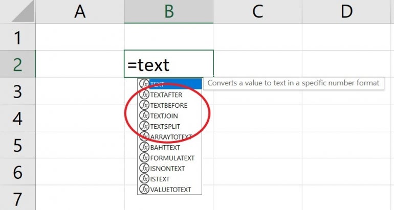
To check, open an Excel workbook and enter =Text into a cell; the AutoComplete should display the new functions, as shown in Figure A. If you don’t see them, and you’re certain that you have Microsoft 365, talk to your administrator.

Figure A

How to use TEXTAFTER() in Excel

Trying to find characters in the middle of another string is one of the hardest string tasks. You have to find the specific character, count all of the characters and subtract the number of characters from the position of the specific character. If you’ve never written one of these expressions before, count yourself lucky because now you won’t have to.

Excel’s new TEXTAFTER() function returns characters that occur after a specified character or string. It renders the above headache null and void.

TEXTAFTER() uses the following syntax:

=TEXTAFTER(text,delimiter,[instance_num], [match_mode], [match_end], [if_not_found])

with only two required arguments:

• text is the string you’re searching.
• delimiter is the specific character that divides the before and after characters.

The remaining arguments are optional and will help you refine the results:

• instance_num is the delimiter after which you want to extract the text. By default, instance_num = 1. A negative number starts searching text from the right. You’ll use this optional argument when the delimiter occurs more than once.
• match_mode determines whether the text search is case-sensitive. 0 is the default and is case-sensitive. 1 isn’t case sensitive.
• match_end evaluates the end of text as a delimiter. 0 is the default, and the text is an exact match. 1 will match the delimiter against the end of the text.
• if_not_found is the value the function returns if it fails to find a match. #N/A is the default.

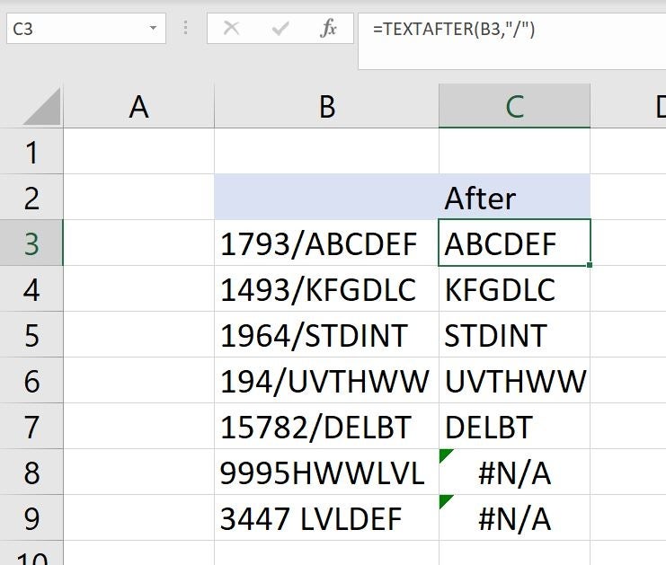
A delimiter is a character that separates characters in a string. If you’re not familiar with this term, you will learn about it in our first example. As you can see in Figure B, the function in C3

=TEXTAFTER(B3,"/")

and copied to the remaining cells specifies the / character as the delimiter. It works for all but two of the strings. Those two strings don’t contain the delimiter at all.

Figure B

The errors aren’t a problem. In fact, they expose inconsistent data, so in this case, I don’t recommend taking any measures to inhibit that error. However, you can use one of the optional arguments to display meaningful information about the error.

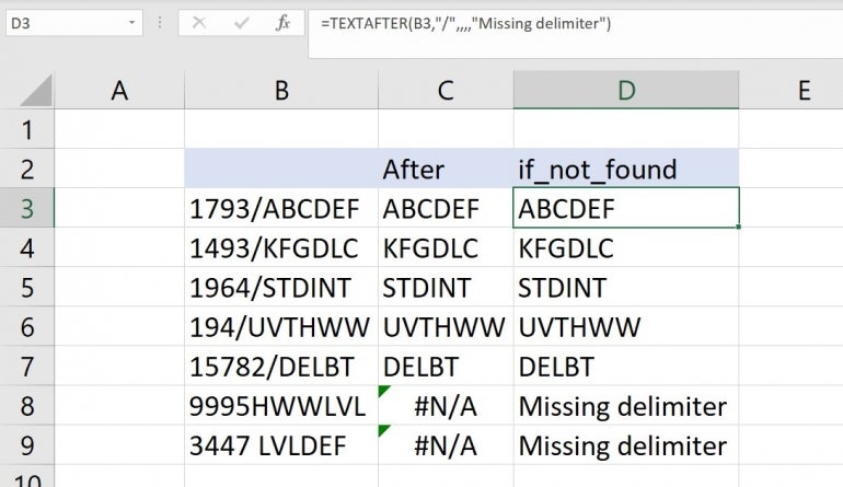
Figure C shows the results of using the if_not_found function as follows:

=TEXTAFTER(B3,"/",,,,"Missing delimiter")

The message “missing delimiter” is specific and more helpful than the error value.

Figure C

Another important argument is instance_num because you’ll often work with strings that contain multiple instances of the same delimiter.

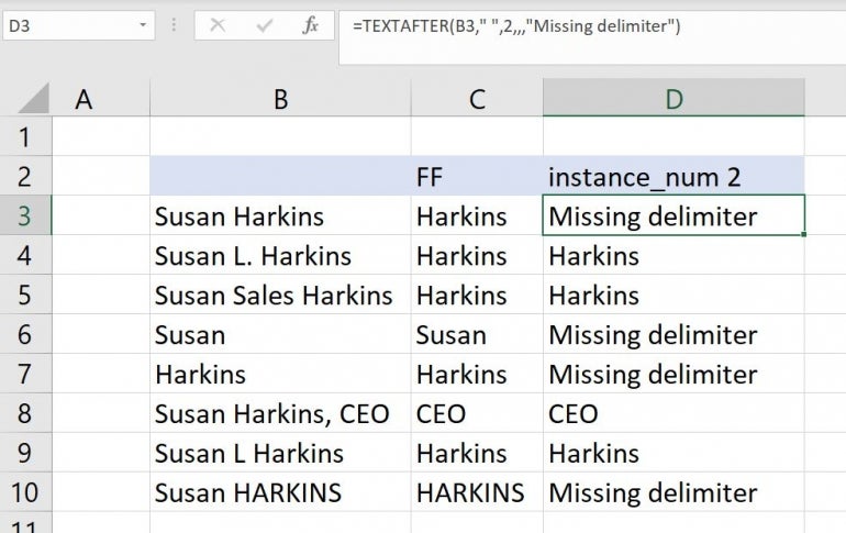
Figure D shows this argument at work in another data set, and it also exposes inconsistent values. Column C shows the results of running Flash Fill to find a pattern that will return only the last portion for comparison. Column D uses TEXTAFTER():

=TEXTAFTER(B3," ",2,,,"Missing delimiter")

Figure D

The value 2 tells the function to return the characters after the second occurrence of the delimiter, which is a space character, represented by ” “. There’s a space character between the quotes. If the string doesn’t have two delimiters, it returns “missing delimiter.” However, one of the strings returns “CEO.” That’s an error the function can’t catch.

You might try the function:

=TEXTAFTER(B3," ",-1,,,"Missing delimiter")

in column E. As you can see in Figure E, it still doesn’t work for the CEO instance; however, it does turn up a surprise: E6 returns nothing.

At first, you might think it’s because the value is a single word, “Susan,” but so is “Harkins” in the next cell, and the function returns “Harkins,” as expected.

Figure E

If you suspect there’s a space character at the end of Susan or Harkins, you’re right. If you remove the space character at the end of Susan, the function returns the error message. If you run into this, you can wrap the text argument in a TRIM() function:

=TEXTAFTER(TRIM(B3)," ",-1,,,"Missing delimiter")

How to use TEXTBEFORE() in Excel

We don’t need another article to demonstrate TEXTBEFORE(). This function is identical to TEXTAFTER() except for the obvious: TEXTBEFORE() returns the characters before the delimiter. Everything else, the arguments, errors and pitfalls are the same.

The downloadable demonstration file contains the same data using TEXTBEFORE(), in case you’d like to see it at work.

Stay tuned

There’s one more new text function, TEXTSPLIT(). I’ll cover this one in a future article.