


Hiding a column tucks data out of sight without interfering with its purpose. You might want to hide confidential data or a helper column. Or, you might want to remove unnecessary columns from a busy sheet. Fortunately, hiding and unhiding columns is easy, with the exception of unhiding column A. In this article, you’ll learn how to hide and unhide columns, as well as the not-so-intuitive steps for unhiding column A.
PREMIUM: Build your skills with this Excel power user guide.
I’m using Microsoft 365 on a Windows 11 64-bit system. However, everything you learn applies to older versions and Excel for the web. Although the article hides and unhides column A, you can apply what you learn to hiding and unhiding row 1.
Jump to:
Selecting a column
Hiding and unhiding a column requires only a few clicks: select the column, right-click and choose the option. However, you must select the entire column(s) beforehand. To do so:
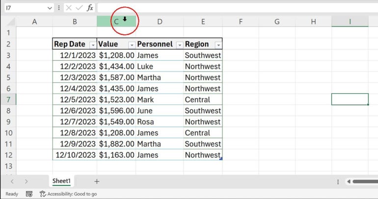
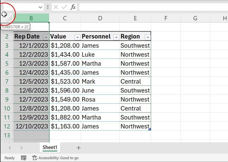
- Hover the cursor over the column’s header cell until it turns into a black pointer (Figure A).
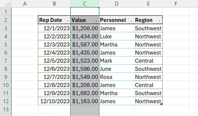
- Click the header cell (column C) to select the whole column (Figure B).
If you want to select multiple columns, select the first column and then drag the selection left or right to add adjacent columns to the selection. To create a noncontiguous selection of columns, select the first column, hold down the Ctrl key and click the header cells for the columns you want to add to the selection.
Now that you know how to select whole columns, let’s move on to hiding a column.
SEE: Explore these Excel tips and tricks for beginners and pros.
Hiding columns in Excel
With column C selected, you’re ready to hide it as follows:
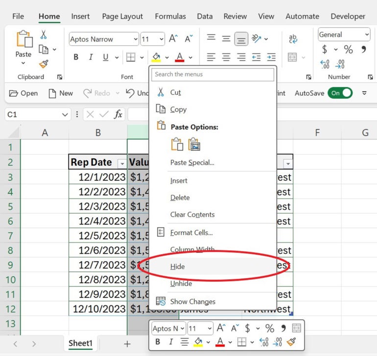
- Right-click the selected column.
- Choose Hide from the resulting context menu (Figure C).
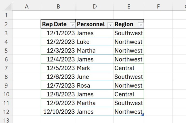
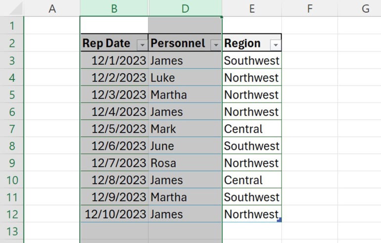
As you can see in Figure D, column C is no longer visible.
Instead of right-clicking, you can also click Formatting in the Cells group on the Home tab, choose Hide & Unhide and then select Hide Columns from the resulting menu.
See: Here’s how to hide rows and columns and use groups in a shared Microsoft Excel workbook.
Unhiding columns in Excel
Unhiding a column isn’t intuitive, but it isn’t difficult. To do so, you select the columns adjacent to the hidden column and then repeat the process to hide the column, choosing the unhide option instead. You’re really selecting three (or more) columns: the hidden column(s) and each column on either side of the hidden column(s).
Let’s unhide column C as follows:
- Select columns B and D by clicking the header cell for column B and then drag the selection to column D (Figure E).
- Right-click the selection.
- Choose Unhide from the context menu.
SEE: Here are some of the best keyboard shortcuts for rows and columns in Microsoft Excel.
Unhiding column A in Excel
So far, the methods for hiding and unhiding columns work fine until you need to unhide column A — there’s only one adjacent column, column B. Selecting just column B won’t also select the hidden column A. But that doesn’t mean column A is gone forever; however, the selection technique will be different.
First, let’s hide column A, so we can then unhide it:
- Click column A’s header cell.
- Right-click the selected column.
- Choose Hide from the contextual menu.
Now it’s time to unhide column A as follows:
- Hover the mouse over column B’s header cell, and drag left. The pointer changes from the selection arrow to a cross (Figure F). This will happen as the mouse pointer nears the Select All cell.
- Right-click, and choose Unhide.