Distinguish business rule violations

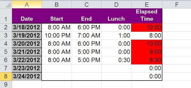
ntUsing conditional formatting, you can spot when something is breaking a business rule. For example, this figure shows a simple timekeeping sheet that highlights a workday that exceeds eight hours. Why? Because your organization requires approval for anything over an eight-hour day.

Distinguish business rule violations

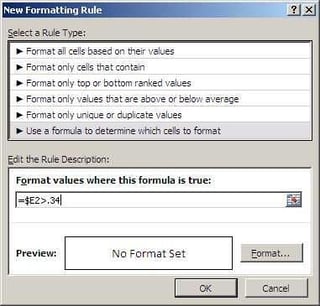
ntAs you can see here, working with the time values complicates things a bit. This solution uses >.34 to represent time values greater than eight hours, which will work in most cases — you can’t use the value 8 or even the time value 8:00. You can also use the predefined Greater Than rule in Excel 2007 and 2010, which will automatically use the more accurate value of 0.333333….

Display simple icons

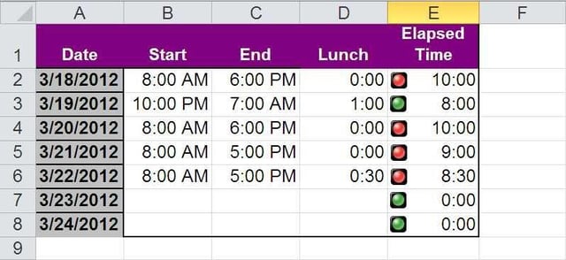
ntUsing conditional formatting (in 2007 and 2010), you can display icons that may be easier to interpret than the values they represent. For instance, a simple checkmark might be quicker to discern than the text value yes, on, true, and so on. Here we have an icon solution for the rule violation we saw earlier.

Display simple icons

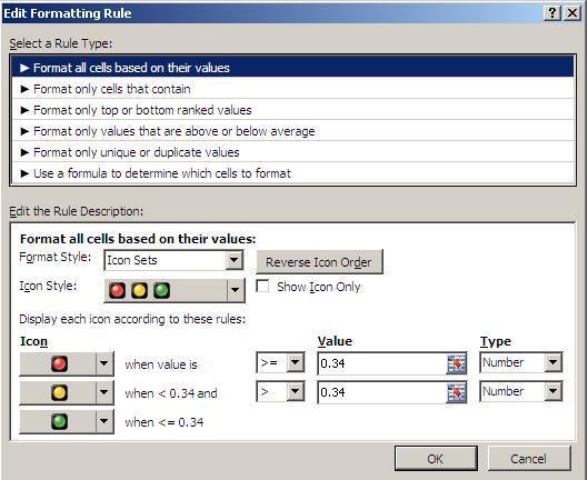
ntTo produce this effect, select the values in column E and apply one of the default icon sets. Then, use Manage Rules to manipulate the results. Make sure you click Reverse Icon Order first.

Highlight a row based on a single value

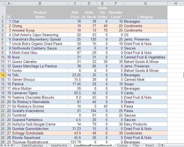
ntFilters are great for limiting what you see, but sometimes you want to compare records. When this is the case, conditional formats can distinguish records. Here’s a data set of products with a conditional format highlighting only Condiment records.

Highlight a row based on a single value

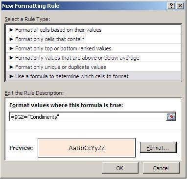
ntSelect the entire data range (not the column headings) so Excel can format the entire record (row). The figure above shows the formula-based settings. The $G2 component creates a relative address, which updates with each row: G4, G5, G6, and so on. When the value in the referenced cell equals the string “Condiment,” Excel highlights the entire row.

Create a dynamic record highlight

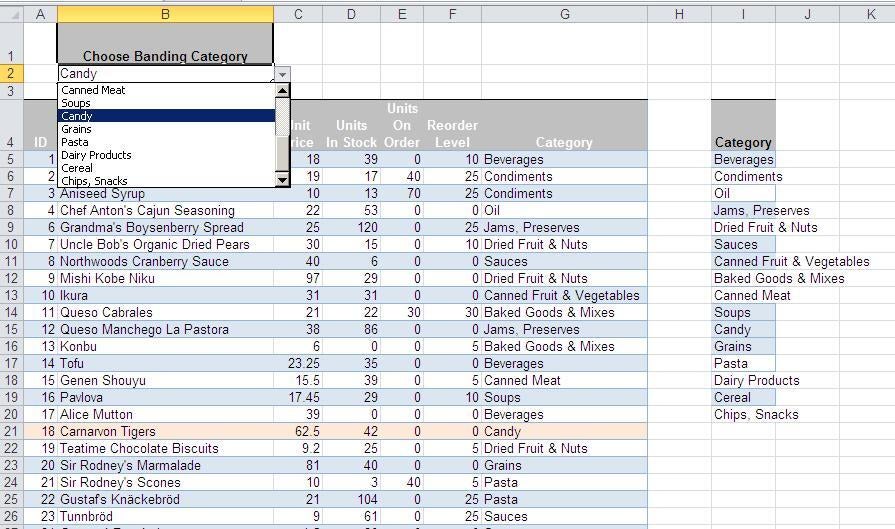
ntHighlighting an entire record is convenient. But what if you want the conditional format to be more… conditional? For instance, suppose you want users to choose the category on the fly.

Create a dynamic record highlight

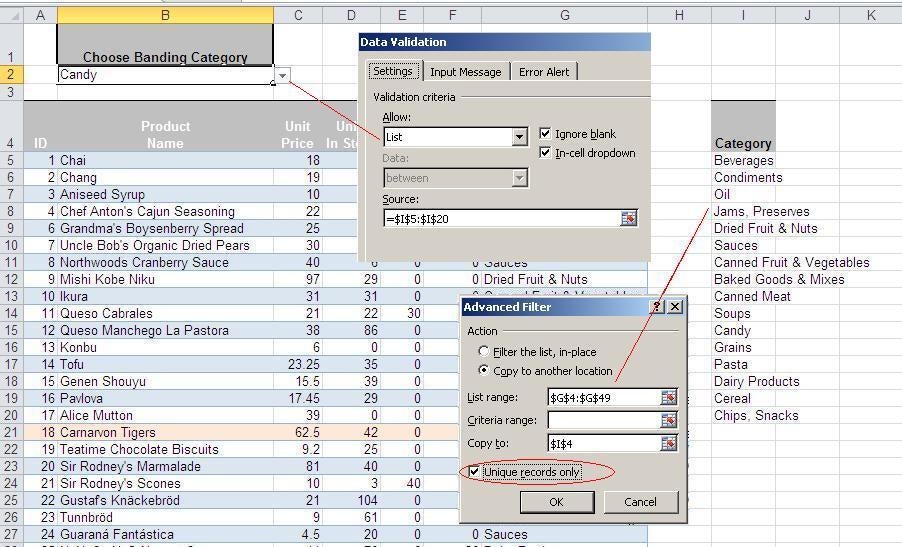
ntFirst, use the Advanced Filter feature to copy a unique list to an out-of-the-way spot. Then, use the Data Validation feature to create a list.

Create a dynamic record highlight

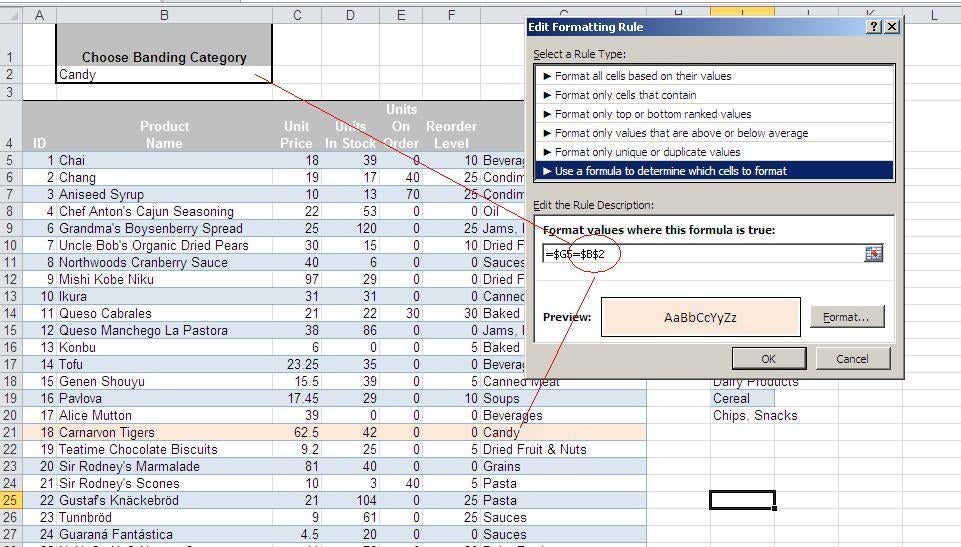
ntWith the list in place, update the conditional format formula to reference the input list cell. Instead of referencing a cell within the row, the formula references the validation list in B2. Selecting an item from the validation list updates the conditional formatting.

Compare values

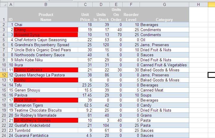
ntSometimes, you need to compare values. For instance, you might track inventory levels by comparing the stock on hand to a reorder level. Using conditional formatting, you can alert users when it’s time to reorder.

Compare values

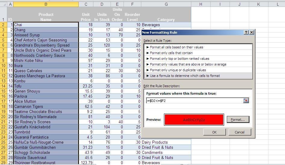
ntSelect the values you want to format — in this case, that’s B2:B46. (You could highlight the entire row or one of the inventory values.) Then, apply the format shown here.

Compare lists

ntYou can find discrepancies between two lists using a conditional formatting rule.

Compare lists

ntThis rule compares each value in column A to its counterpart in column B. If they’re not the same, Excel highlights the value in column A. To highlight the values in column B instead, select the values in column B and update the rule formula to reference the values in column A.

Create alternating bands

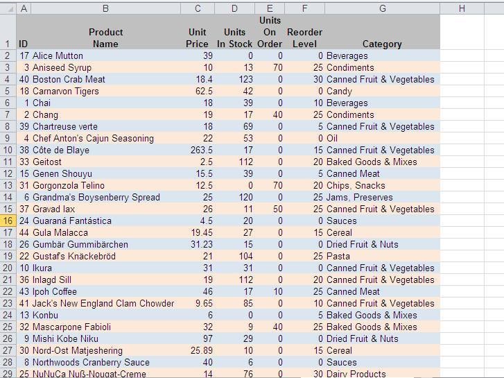
ntMany sheets highlight every other row (banding) to improve readability. The Table feature offers several predefined formats that include bands, but you end up with a table instead of a plain data set. When you don’t want a table, use conditional formatting to create alternating bands.

Create alternating bands

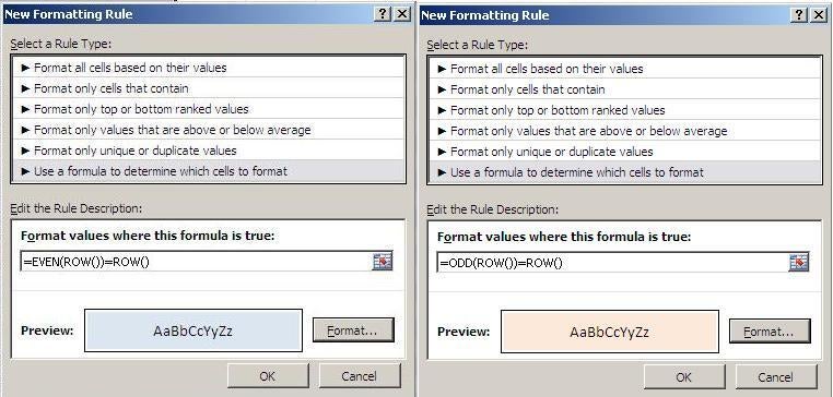
ntThe rule shown here highlights cells to achieve the alternate band effect.

Find duplicates

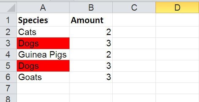
ntTo find duplicate values or records, you can use a filter, but conditional formatting can pinpoint duplicate values on the fly. For instance, this sheet shows duplicate values in a single column.

Find duplicates

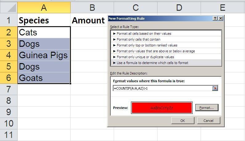
ntSelect the values you want to format and apply the formula-based rule shown here.

Find duplicates

ntTo ignore the first occurrence and highlight only subsequent values, use this formula:

n

=COUNTIF($A$2:$A2,A2)>1

n

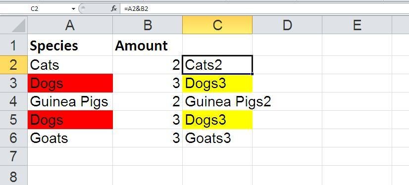
ntIf you want to check for duplicate values across multiple columns, concatenate the values and apply a similar rule to the results, as shown in the figure above. You can also hide duplicates (which I don’t always recommend) by selecting a font color that matches the sheet’s background.

Find discrepancies

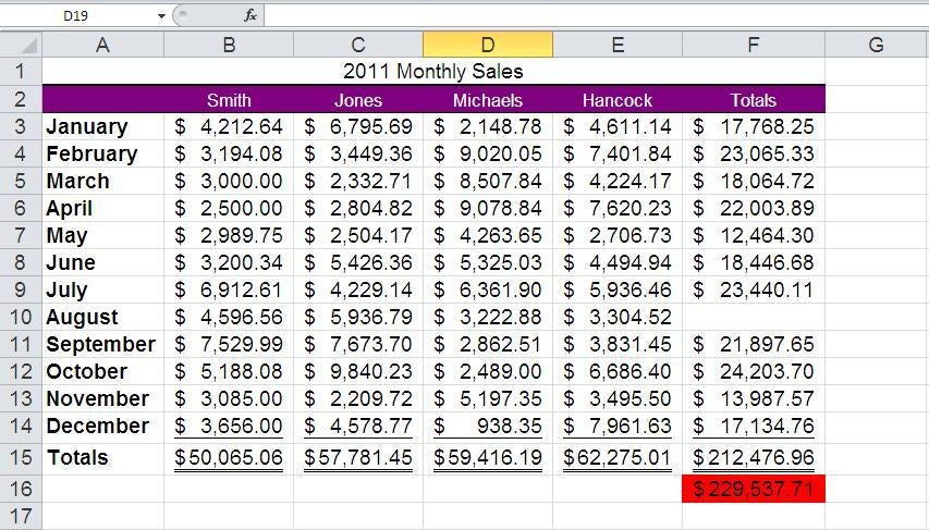
ntVerifying data is an important task, and Excel’s conditional formatting can help by alerting you to inconsistencies. The figure above shows a common accounting tool known as cross-footing — the process of double-checking totals by comparing subtotals across rows and columns — in cell F16. Adding the conditional format makes the discrepancy hard to miss when the two totaling values don’t match.

Find discrepancies

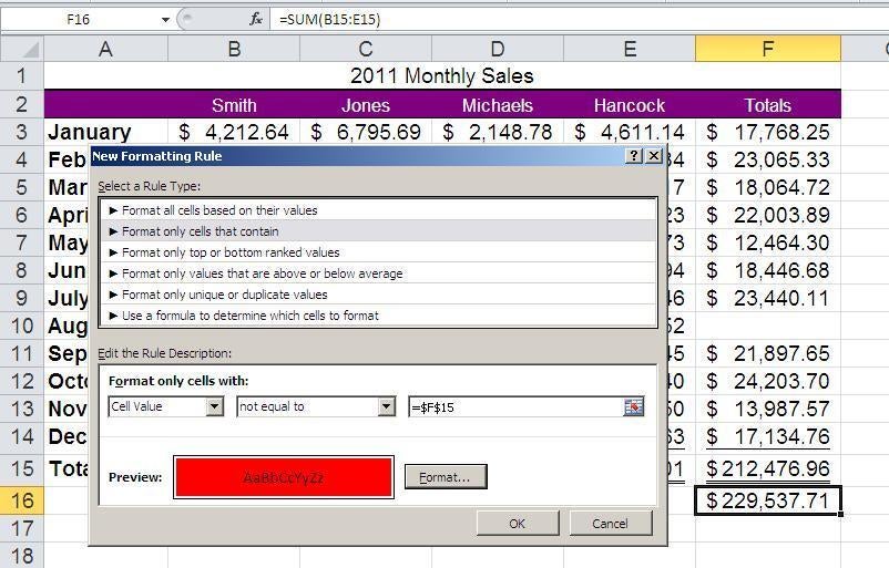
ntSelect either of the cross-foot formulas and apply the rule shown here.

Find the smallest or largest duplicate

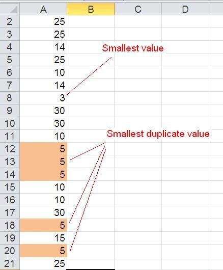
ntAs you can see above, the value 3 is the smallest value in the column, but Excel highlights each occurrence of the value 5.

Find the smallest or largest duplicate

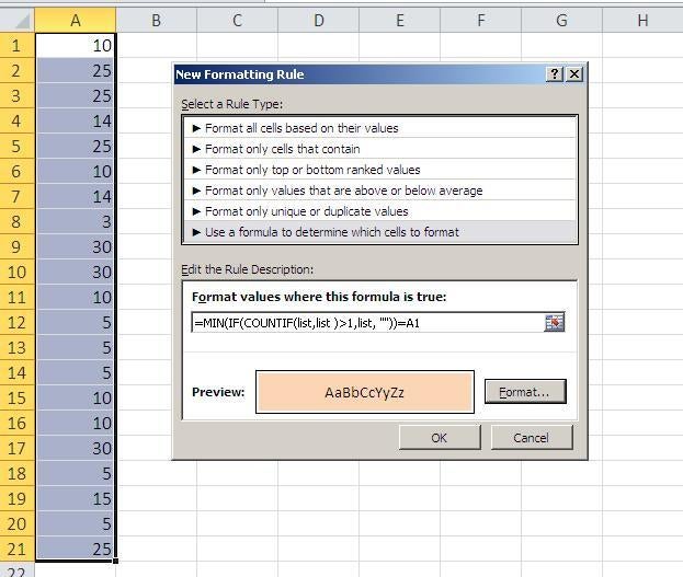
ntThis rule is unstable if you use normal referencing, so apply a range name to your data set before applying the conditional formatting rule. The rule shown here will highlight the value 3 in the range named List only if 3 is also a duplicate. (To find the largest duplicate value, substitute the MIN() function with MAX().)