10 obscure Excel tricks that can expedite common chores
Image 1 of 19
1: Select All with one click
This gallery is also available as a TechRepublic article and PDF download.
Over the years, each new version of Excel has introduced some nifty features. However, buried within Excel are lots of cool features that too few users have discovered. If you (or your users) perform certain tasks every time you use Excel, you’ll want to make sure you’re taking advantage of these time-saving shortcuts.
Version note
These tips apply to Excel 2003, although most of them work the same way in earlier versions of Excel.
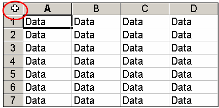
The next time you need to select an entire worksheet, click the little gray box in the top-left corner of the sheet. It’s the space above the row numbers and to the left of the column letters.
Why would you want to select the entire worksheet? Let’s count some of the ways:
- With the entire worksheet selected, you can copy it from one workbook (XLS file) and then paste it into a worksheet in a different workbook. Selecting the whole worksheet ensures you won’t accidentally miss something. Note: If you want to make a copy of a worksheet within the same book, just right-click on the worksheet tab, choose Move or Copy, then select the Create A Copy check box.
- With the entire worksheet selected, you can quickly and easily change the font in all cells or apply formatting to all cells.
- With the entire worksheet selected, you can double-click on any line separating two column letters or the line separating any two rows. Doing so tells Excel to adjust the width of the columns or the height of the rows to accommodate the data in the cells, which is very helpful if you’ve just shrunk (or enlarged) the font size of the text in your cells.
- There are, of course, other ways to select all the cells in a worksheet. If you’re a keyboard person, press [Ctrl]A. If you’re a menu person, go to Edit | Select All.

2: Copy the formatting (attributes) of one or more cells and apply them to another cell or range
2: Copy the formatting (attributes) of one or more cells and apply them to another cell or range
Once you learn to use the Format Painter tool (which looks like a little yellow paintbrush on the Standard toolbar), you’ll wonder how you ever got by without it. To format a cell (or cells), select a cell (or cells) that are formatted the way you like and click Format Painter. Then, click and drag to apply that formatting to another cell (or range of cells).
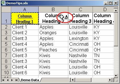
Here’s an example to illustrate how Format Painter works. Start by manually formatting cell A1 as Times New Roman 9, bold, and underlined and then use the Fill Color tool to make the background of the cell yellow. With cell A1 selected, click Format Painter. You’ll notice that Excel displays a paintbrush next to the cursor.
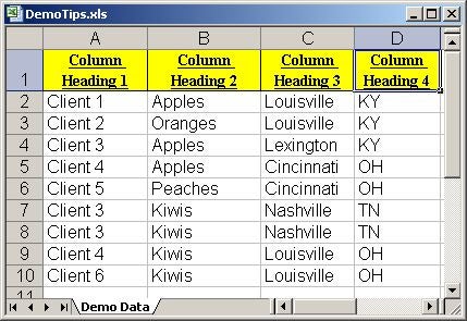

After you pick up the formatting of a cell, click on any other cell or drag through a range or cells to "paint" the cell(s) with the same formatting
After you pick up the formatting of a cell, click on any other cell or drag through a range or cells to "paint" the cell(s) with the same formatting
While that paintbrush is visible, all you have to do is click (and/or drag) to apply all of the attributes from cell A1 to any other cells. This shortcut saves time because you don’t have to manually reapply the font and other attributes to other cells.
Note: By default, Format Painter is a “once and out” function. That is, if you click once on Format Painter and then paint a cell or range of cells, Excel will stop painting as soon as you release the mouse. If you want to paint a number of different cells or range of cells, double-click on Format Painter. The paint brush function will then continue painting cells as long as you keep clicking. To turn off Format Painter after you’ve double-clicked it, press [Esc].
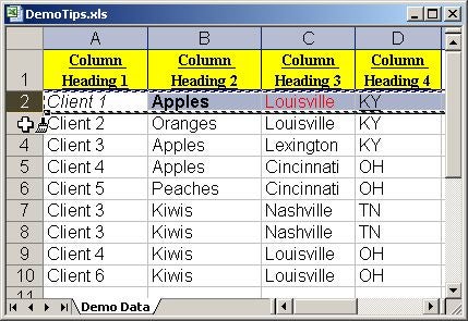

If you apply different formats to multiple cells, you can paint all those formats at one time by selecting the row before you click Format Painter
If you apply different formats to multiple cells, you can paint all those formats at one time by selecting the row before you click Format Painter
The cool thing about Format Painter is that it isn’t limited to picking up the attributes of one cell at a time. For example, suppose you have applied different formatting attributes to two or more cells in the same row or column, as we did in Row 2.
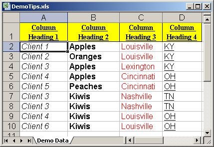

Select a row or column, click Format Painter, and then paint other rows and columns; Excel will format the destination cells in the same pattern as the cells in the original row or column
Select a row or column, click Format Painter, and then paint other rows and columns; Excel will format the destination cells in the same pattern as the cells in the original row or column
Using Format Painter, you can transfer all those formats to the rows above.

3: Perform one-click data mining with AutoFilter
3: Perform one-click data mining with AutoFilter
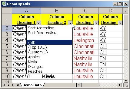
If you support Excel users, AutoFilter will be a surefire hit, both for beginners and for experienced users who haven’t seen this feature in action before. Go to Data | AutoFilter, and Excel will add drop-down arrows to the first cell in each column of data in your sheet. When you click on any of those drop-down arrows, Excel will display a list of the unique entries in that column.
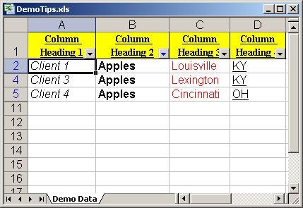

When we select Apples from the AutoFilter drop-down list for column B, Excel hides all records except those that match our selec
When we select Apples from the AutoFilter drop-down list for column B, Excel hides all records except those that match our selec
Just select the desired entry to limit the display of records.
AutoFilter notes
If you look closely, you’ll notice that the color of the drop-down arrow changes from black to blue whenever you make a selection. That change in color is a visual cue to remind you that your list has been filtered by a selection from that column.
As you probably guessed, you aren’t limited to filtering the list on just one column. You can click on the drop-down for two or more columns, and Excel will display only those records that match your selections in each column.
There are two ways to turn off AutoFilter. One is to click on each of the columns where you made an AutoFilter selection and choose the (All) option. The other way is to go to Data | Filter and select Show All.

4: Press [Ctrl]~ to display formulas so you can troubleshoot or debug them
4: Press [Ctrl]~ to display formulas so you can troubleshoot or debug them
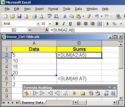
If you wanted to troubleshoot a formula in early versions of Excel, you had to click on the cell containing the formula and look at the formula itself in the Formula Bar. In more recent versions of Excel, you can display your formulas by pressing [Ctrl]~. If you want to view the dependent cells for a particular cell, select it before you press [Ctrl]~.
To demonstrate this feature, open any worksheet that contains at least one formula and press [Ctrl]~. Our sample sheet contains two SUM functions. This screenshot shows our sheet after we selected cell B2 and then pressed [Ctrl]~. Notice that when you press this key combination, Excel 2003 also displays the Formula Auditing toolbar.

5: Generate a unique list of entries in a column
5: Generate a unique list of entries in a column
When you support or teach Excel users, one of the most common questions you’ll hear is, “I’ve got a list with a thousand entries in a column, and many of those are duplicates. How do I generate a list of the unique entries in that column?”
rnThere are at least two good answers to that question. The first answer is to refer back to Tip 3 above: Go to Data | AutoFilter and then click the drop-down list for the column in question. Doing so lets you see the list of unique entries onscreen. If seeing the list satisfies your need, you’re finished.
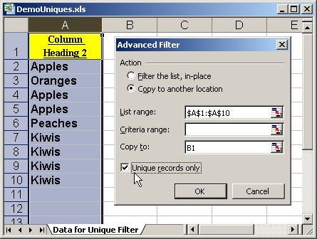
rnThe second answer is the one to use if you want to have a list of the unique entries you can copy and paste elsewhere. To generate such a list, you’ll use Data | Filter | Advanced Filter. To demonstrate how it works, we’ll use the data in Column B from the sample sheet we introduced in the second screenshot.rn
- rn
- Click on the column letter to select the entire column that contains your data and then copy it by pressing [Ctrl]C, going to Edit | Copy, or clicking the Copy button on the Standard toolbar. (Select the whole column because you’ll need the column header.)
- Paste that data into a column away from your source data range or in a new sheet. After you paste the data, it will still be selected. However, if you inadvertently deselect it, just make sure the cell pointer is located anywhere in the data you pasted before you proceed. Note: You don’t have to select all the data or sort it first for this tip to work.
- Go to Data | Filter | Advanced Filter.
- By default, Excel will suggest filtering the list “in-place.” There’s nothing wrong with that, but I recommend copying the unique records to another location, so you can compare the two lists side by side.
- Select the Copy To Another Location option, select the Unique Records Only check box, and type B1 in the Copy To field.
- Click OK, and Excel will copy the unique entries from the source column into the new location. It will even sort those entries in alphabetical order, as shown in the next screenshot.
rn
rn
rn
rn
rn
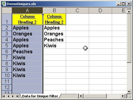

The Advanced Filter feature copied a sorted list of the unique entries from the source data in Column A
The Advanced Filter feature copied a sorted list of the unique entries from the source data in Column A

6: Let Excel calculate your subtotals for you
6: Let Excel calculate your subtotals for you
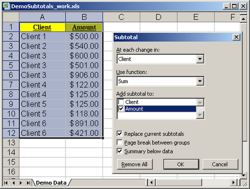
The Subtotals feature is yet another life-changing tool for those who haven’t seen it before. In the old days, before the Subtotals feature was introduced, here’s how you generated subtotals: You’d sort your data, manually insert blank rows between the groups of data you wanted to subtotal, and manually insert the appropriate Sum functions. Many Excel users still take that approach when they want to generate subtotals, which is regrettable, since it provides many opportunities for errors.
Here’s a quick walk-through of how to use Excel’s Subtotals feature:
- rn
- Save your worksheet under a work name. To do so, go to File | Save As and add “_work” to the original filename. Trust me, you don’t want to practice using the Subtotals function using the only “good” copy of your worksheet. As you’ll find when you sally forth into experimenting with this feature, a misstep can make a mess of your data that’s hard to clean up.
- Sort your data on the column by which you want to subtotal. This is an important step, because the Subtotals feature doesn’t care if your data is sorted; it will simply subtotal records in the order they appear.
- Click anywhere in your source data and go to Data | Subtotals. When you do, the Subtotal dialog box will appear and Excel will take its best guess as to the column on which you want to subtotal and the function you want to use (Sum) for those subtotals. (You can also generate subtotals using a host of other functions, such as Average, Min, and Max.)
- Click OK to generate the subtotals.
rn
rn
rn
rnThis screenshot shows what our sample data looked like before we generated the subtotals. The next screenshot shows the results.


Here's what our worksheet looks like after we generated subtotals of Amount by Client
Here's what our worksheet looks like after we generated subtotals of Amount by Client
Note: The Subtotals function doesn’t automatically expand the width of the columns to accommodate the subtotaled amounts or the labels. We had to widen our columns before we captured the screen shot of our worksheet to display the contents of columns A and B.


Here, we opted to display only the subtotal and grand total rows
Here, we opted to display only the subtotal and grand total rows
At this point, direct your attention to the top-left corner of the worksheet. You’ll see, in an extremely tiny font, the numerals 1, 2, and 3. If you want to see only the grand total line, click 1. Click the number 2, and Excel will “roll up” the detail lines and display only the subtotal and grand total rows, as shown in Figure M. Click 3 to display the default view, which is all of the details rows, the subtotals, and the grand total.
Subtotals notes
If you want to view the detail rows for just one of the entries in your list, click the plus sign ( ) beside that row. To remove the subtotals and restore your worksheet to its original state, go to Data | Subtotals and click the Subtotal dialog box’s Remove All button.

7: Analyze selections with the AutoCalculate menu
7: Analyze selections with the AutoCalculate menu
This is a handy tip for anyone who teaches spreadsheet skills classes to adult learners. I use this tip to open my Excel classes, and I have been surprised at how many experienced Excel users have never heard of it.
rnHere’s how it rolls. Create a new workbook and enter some random text and numbers. Press the NumLock key and confirm that you see NUM displayed in Excel’s Status bar at the bottom of the Excel window.
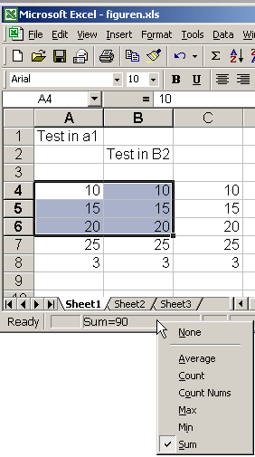
rnRight-click in the vicinity of Ready in the bottom-left corner of Excel’s Status Bar to display the incalculably valuable AutoCalculate menu. Gone are the days when you manually key a few numbers off of a sheet to get a quick total. Now you can get it off the screen with a few clicks.
rnTthe AutoCalculate menu calculates results on the fly and saves you the trouble of setting up formulas to calculate things like the sum, minimum, maximum, or average values in the cells you’ve selected.
rnIf you want to have fun, activate any of the AutoCalculate menu options. Then, click and roll through a range of cells that contain various entries and watch as Excel displays the changes in the current calculation on the Status Bar.
rnIt’s a nice little feature whose only drawback is that you can’t copy and paste the results of the calculations. It’s dynamic and view-only. Still, it’s great for sanity checks. For instance, you might be looking to the Count for what should be the number of expected data rows plus the row for the column head. Just click on a column head, and AutoCalculate will tell you how many cells in that column contain values.
8: Love your [Ctrl] key--for three reasons
This three-fer will demonstrate why you should love and use your [Ctrl] key:
Reason 1–Fast navigation.
When you press [Ctrl] and any arrow key (north, east, south, or west), you jump to the last populated cell in that direction. Think of using the [Ctrl]-arrow key shortcut as an alternative to pressing [Page Down] to find the bottom row of a data set or pressing [Tab] to find the last column. Bonus tip: Hold down the [Shift] key while you press any [Ctrl]-arrow key shortcut to select all the cells between where you are and where you jump with the [Ctrl] key.
Reason 2–You can make noncontiguous selections.
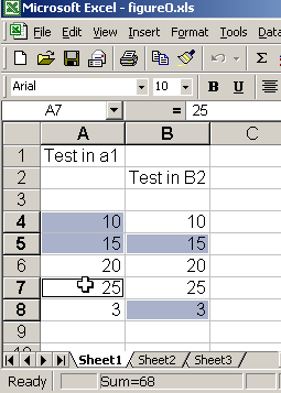
That’s a fancy way of saying you can select any cells you want, regardless of whether they’re contiguous–next to each other in a row or column. Hold down the [Ctrl] key while you click on a cell or click and drag through a range of cells. As long as you hold down the [Ctrl] key, you can click and select to your heart’s content.
Combine this tip with tip Number 7 and you can use the AutoCalculate tool to analyze any combination of individual cells or blocks of cells. This screenshot shows our screen when we used AutoCalculate to sum the cells we selected while holding down the [Ctrl] key.
Reason 3–Fast data entry.
Suppose you want to put the same string, number, or formula into two or more cells. Using the old-fashioned approach, you’d type the string, number, or formula into the first cell and then copy and paste that entry into the destination cells. But there’s a little-known time-saving tip that makes short work of placing the same entry in multiple cells. First, select all the cells you want to populate. Type the entry, but don’t press [Enter]. Instead, press [Ctrl][Enter]. When you do, Excel will copy what you typed into all of the selected cells.

9: Transpose data from a row to a column, or vice-versa
9: Transpose data from a row to a column, or vice-versa
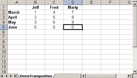
Here’s a tip that eliminates the need to rekey data. Suppose you’ve entered your data with three column headings running across Row 1 and three row headings running down Column A, like the ones shown above.

The Transpose option lets you rearrange your data with just a few clicks
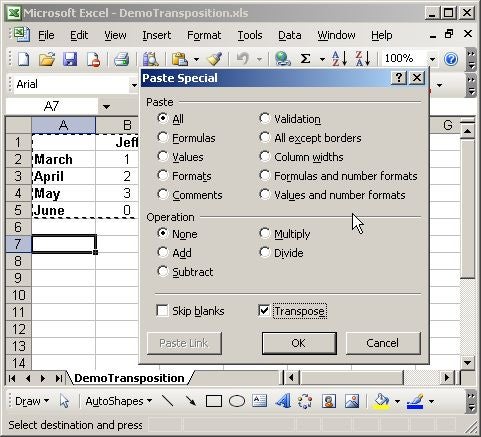
The Transpose option lets you rearrange your data with just a few clicks
After working with the data for a while, you decide you’d rather have the current set of row labels (months) running across the columns. Whatever you do, don’t even think about rekeying the data.
You’ll find the best solution under the Paste Special menu. Start by selecting and copying your entire data range. Click on a new location in your sheet, then go to Edit | Paste Special and select the Transpose check box.
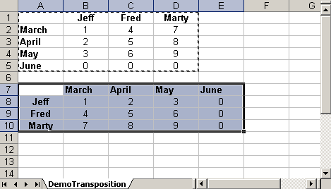

Here's what our data looks like after we copied and pasted our data using the Paste Special | Transpose option
Here's what our data looks like after we copied and pasted our data using the Paste Special | Transpose option
Click OK, and Excel will transpose the column and row labels and data, as shown above.
Note:You aren’t limited to using the Paste Special | Transpose option to rearrange multiple rows and columns of data. It works just as well when you need to turn a single row of labels into a column, or vice-versa.
10: Convert calculations to literal values
This jewel, like Tip 9, is also found under Edit | Paste Special. Experienced users may squawk that this tip doesn’t qualify as obscure. However, I decided to include it because, in teaching both beginning and advanced Excel classes to thousands of adult learners over the years, I’ve met too many people who never even heard of it–which is a crying shame.
Here’s how it works. Suppose you have a worksheet with columns and rows chock full of calculations, running the gamut from Sum functions to If tests to vertical and horizontal lookups. The calculations are correct and your data is pristine. You save the worksheet.
Now you need to use a subset of that worksheet in another worksheet. If all you’re going to do is print the subset of columns or rows, you can simply hide those rows and columns, print what you need, and unhide the columns and rows later to restore the sheet to its normal state.
But if you’re going to e-mail a copy of the spreadsheet to a coworker or a third party, you may not feel comfortable simply hiding certain rows and columns. You may want to delete them instead. The problem is, of course, if you simply start deleting rows and columns, you’re going to get error messages in the cells that depend on the cells you deleted.
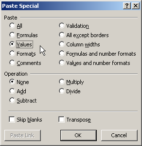
The solution? First and foremost, save a copy of your pristine spreadsheet under a new name. Just go to File | Save As and add “_work” to the end of the “real” name. Use the Select All tip (1) to select the entire sheet and then copy it. Without moving the cursor, go to Edit | Paste Special. Now, select the Values option, as shown above,and click OK. When you do, Excel will replace all the formulas with the values they’re currently calculating and displaying. At that point, you can delete columns or rows and move cells around without generating a single error message.
Note: If you use the Paste Special | Values option and the data you’re pasting contains calculated dates or numbers formatted as currency, the date calculations will be pasted as the Julian date value, and the currency will lose its dollar signs and commas. To preserve that kind of formatting when you convert calculations to literals, simply choose the Values And Number Formats option (instead of Values).
