Performing common Excel tasks in OpenOffice.org 2.0's Calc

DataPilot provides you with an easy way to ferret out information hidden in a spreadsheet

This gallery is also available as a TechRepublic article.

Many folks may be a bit apprehensive about making the switch from Microsoft Office to OpenOffice.org because of the learning curve. Sure the cost difference, several hundred bucks verses free, is very, very attractive! But is that savings going to be eaten away by training costs and lost productivity? Fortunately, the answer is no! OpenOffice.org 2.0’s cadre of open source developers has spent a great deal of time in an attempt to make the two office suites as alike as possible in both the feature set and more importantly in the user interface. And by and large, they’ve succeeded!

Realistically speaking, it will take some time to make the transition as many features and settings are named differently and are in different locations, but the names and locations aren’t too far of a stretch of the imagination and it’s easy to make the connections. As such, it won’t take nearly as much time as you might think for seasoned Microsoft Office users to train themselves how to use OpenOffice.org 2.0.

Of course every business generates data of some sort and since the early days of Lotus 1-2-3, business people have been have been entering and manipulating data in electronic spreadsheets. When it comes to this application, OpenOffice.org 2.0’s Calc provides you with everything you need and then some. With this in mind, let’s take a look at performing some common Excel tasks in OpenOffice.org 2.0’s Calc.

Massaging numbers with the DataPilot

While the object of putting numbers into a spreadsheet is to make it easier to analyze the data, often times important trends or even problems can become buried deep with the numerous rows and columns of a huge spreadsheet. In order to help you ferret out that hidden information, filter it, and then explore it from a number of angles Calc provides you with a feature called DataPilot, which of course is designed to be emulate Excel’s PivotTable feature.

To see how DataPilot works let’s suppose that you have a spreadsheet that contains sales data for 26 products in a catalog. Each line in the spreadsheet contains the product name, the product category, product price, quantity sold, the sales representatives name, and the total sales figure for that product. While this spreadsheet is very informative as it is designed, suppose that you want to calculate the sales total for each rep?

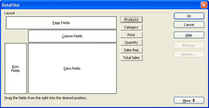
With DataPilot, you can extract this information easily. To begin, select all of your data including the column titles. Next, pull down the Data menu and select the DataPilot | Start command. When you see the Select source dialog box, just click OK. At this point you’ll see the Data Pilot dialog box, which contains a layout template and buttons labeled the same as your spreadsheet’s column titles, as shown above. Now, drag the Sales Rep button and drop it on the Row Files section of the template, Then, drag the Total Sales button to the Data Fields section.

When you click OK, Calc will generate a new table, based on the layout configuration, that contains a list of each of the sales reps and their respective sales totals, as shown above. This information is in the larger spreadsheet, but it isn’t easily discernable.

The Filter dialog box allows you to dig deeper into the data that you've extracted from the larger spreadsheet

If you want to see other trends in this new table, you can click the Filter button right above the table and use the settings in the Filter dialog box to extract other information. For example, you might want to find out who had the most $25 sales, as shown above.

The AutoFormat Chart wizard makes creating charts in Calc a snap

Creating charts

As any spreadsheet guru will tell you, being able to translate your data into a visual display allows you to make an instant impact when presenting your analysis to colleagues. By starting out with a chart, the actual numbers seem to be more intriguing and creating Charts in Calc is a snap. Unfortunately Calc’s graphics rendering engine leaves a little to be desired when compared to Excel, but it gets the job done.

You’ll begin by selecting all of your data including any column and row titles. Next, pull down the Insert menu and select the Chart command to display the AutoFormat Chart wizard, as shown above. If you want Calc to use the values from the first row and column as labels for the chart’s X- and Y-axis, select the First Row As Label and the First Column As Label check boxes. In order to have as much room as you can for the chart, use the Chart Results In Worksheet drop-down to select an available sheet.

The AutoFormat Chart wizard provides a preview pane so you can keep tabs on your chart

As you progress through the AutoFormat Chart wizard you can select from a number of standard chart types, choose a variant of that chart type, and add a title. As you work through this initial design phase, the AutoFormat Chart wizard will display a preview of your chart, as shown above, so that you have an idea what the end result will look like as you select options. When you finish, you’ll have a rather small, basic chart that you can begin spicing up. To begin with, you can use the handles to stretch the chart horizontally and vertically to make it larger.

With the options in the 3D Effects dialog box, you can create a very nice looking chart to display your data

With the chart selected you can pull down the Format menu and let loose with the plethora of options for customizing the axis, the grid lines, the walls, the floor, as well as the background. If you’ve selected a 3D chart variant, then you’ll want to select the 3D Effects command and investigate all the options the 3D Effects dialog box has to offer. Here you can adjust geometry effects, as well as shading and illumination, just to name of few.

Keep in mind that tinkering with all these settings can take a while, but the end result can be quite nice, as shown above.

Using grid lines makes it easier to keep track of data on a printed copy

Printing spreadsheets

Once you’ve developed a spreadsheet in Calc, chances are good that you’ll need to print it for inclusion in a paper report. When you do so, you’ll probably want to include grid lines, customize the footers, as well as have your column titles printed on each page.

To include grid lines, you’ll pull down the Format menu, select the Page command, and when the Page Style dialog box appears, select the Sheet tab. Then, in the Print section, select the Grid check box, as shown above.

You use the Custom Footer buttons to add such things as document title and page numbers to the footer

Keep in mind that if your spreadsheet is wider than a single piece of paper, you can use the Left To Right, Then Down setting in the Page Order section to print the first section of columns, across all the rows and then print the next section of columns.

To customize the footer, select the Footer tab and click the Edit button. You can then use the Custom Footer buttons to place items in the three area panels, as shown above.

Clicking the Shrink button allows you to easily access the spreadsheet and select the column titles

To specify that your column titles are printed at the top of each page, pull down the Format menu, select the Print Ranges command, and when the Edit Print Ranges dialog box appears, click the Shrink button in the Rows to Repeat section, as shown above. Once the Edit Print Ranges dialog box shrinks, select the cells or rows containing your column titles. Then click the Shrink button again.

As you preview the printed page, you can access the Page Style dialog box by clicking the Page button

To see how your spreadsheet will look before you actually print it, click the Page Preview button on the toolbar. If, as you study the mock-up, as shown above, you decide that you want to set other options, just click the Page button and the Page Style dialog box will appear right over top of the Preview window. You can then easily toggle back and forth as you customize the printed copy of your spreadsheet.

Calc makes it easy to export your spreadsheet as a PDF file and attach it to an e-mail message all in one step

Exporting to PDF format

If you want to electronically share the spreadsheet that you’ve generated in Calc with colleagues and don’t want to allow anyone to alter the data, Calc provides you with a feature, that at this point, Excel doesn’t provide–the ability to save the spreadsheet as a standard Portable Document Format (PDF) file. Just click the Export Directly As PDF button on the standard toolbar, type a filename in the Export dialog box, and click the Save button. You can then copy the PDF file to any location you want.

If you’ll be e-mailing the PDF, save yourself a step and select the Send | Document as PDF command from the File menu. You’ll then see the PDF Options dialog box, as shown above, and can optimize the PDF file for sending via email. Calc will then launch your email application, create blank new message, and then attach the PDF.