Microsoft Excel PivotTables are a great way to summarize data. They’re easy to create and they display information in meaningful ways, such as subtotals and grand totals for sums, counts and averages. The article, How to display multiple subtotal rows in a Microsoft Excel PivotTable shows you how to insert multiple subtotal rows into a PivotTable without repeating data. In this tutorial, I’ll show you how to add multiple grand totals to a PivotTable.
SEE: Google Workspace vs. Microsoft 365: A side-by-side analysis w/checklist (TechRepublic Premium)
I’m using Microsoft 365 on a Windows 10 64-bit system, but you can use older versions of Excel. Excel for the web supports PivotTables. You can download the Microsoft Excel demo file for this tutorial.
How to create a PivotTable in Excel
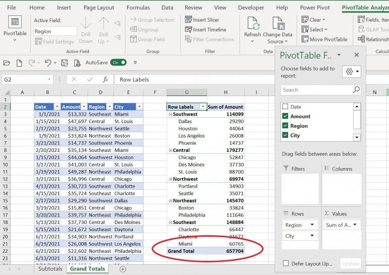
Let’s suppose you track sales for several cities across the US and you want to see subtotals for regions. Figure A shows the source data and the first PivotTable you might design. As you can see, by default, Excel displays a SUM() function for subtotals and grand totals, but you might run into situations where you need more than one grand total.
Figure A

To create this PivotTable, click anywhere inside the data source Excel Table and then do the following:
1. Click Insert.
2. Inside the Tables group, click PivotTable.
3. In the resulting dialog, click Existing Worksheet, and then click G2 in the Location control.
4. Excel will insert a blank frame. Using the fields list shown in Figure A as a guide, build this PivotTable by dragging fields to the appropriate sections.
The grand total at the bottom is a sum, by default. Let’s add a second grand total row that shows the average sale.
How to add multiple grand total rows to a PivotTable in Excel
When you create a PivotTable, Excel will insert a grand total at the bottom that returns the sum of the value column. Sometimes, you might need a second or even multiple grand total calculations, such as sum, average and so on.
The good news is that you can display multiple grand totals. The bad news is that the process isn’t intuitive, and it requires several steps.
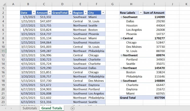
To begin, return to the source data and add a column (Figure B). Change the heading to GrandTotal and leave the data cells empty. To insert the column, right-click column D’s (Region) header cell and choose Insert from the resulting submenu. I purposely omitted the space character between Grand and Total to make it easier to differentiate between this new grand total row and others.
Figure B

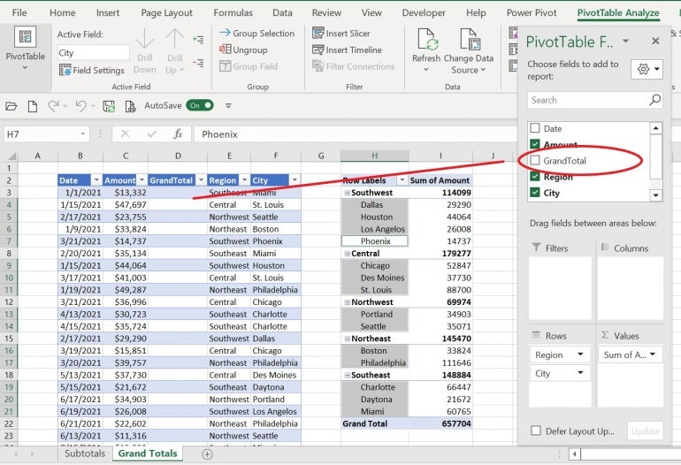
Right-click any cell in the PivotTable and choose Refresh to add the new field (Figure C).
Figure C

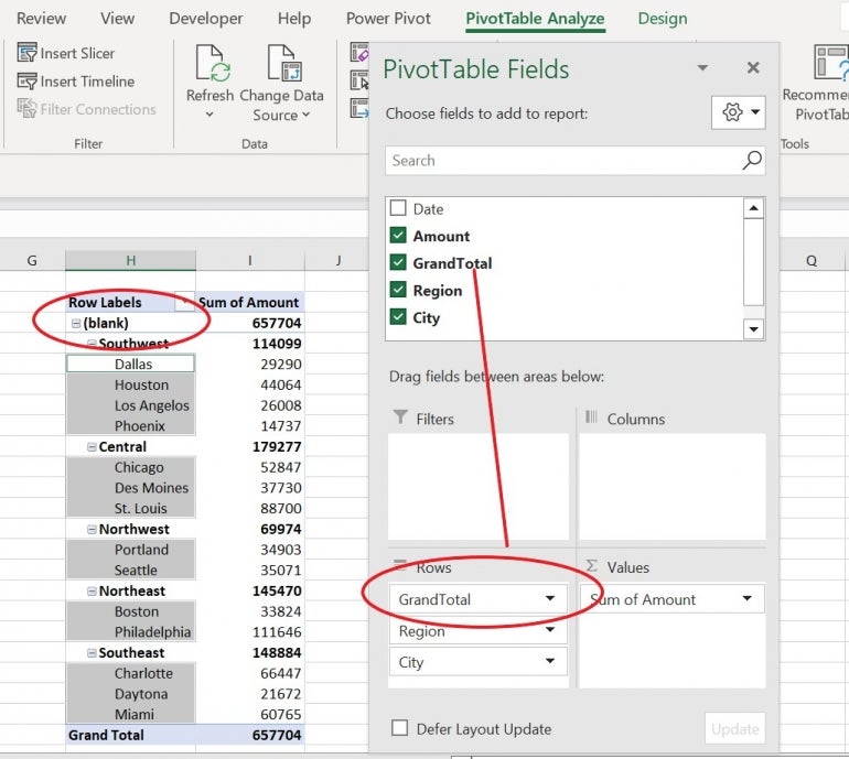
Drag the new GrandTotal field to the Rows list, making sure it’s at the top of the list (Figure D). The result is a new row at the top of the PivotTable. The region cell displays (blank) and the amount cell displays the same thing as the grand total row at the bottom does, 657704. Otherwise, nothing else changes.
Figure D

Next, move the new row to the bottom of the PivotTable as follows:
1. Click inside the PivotTable and click the contextual Design tab.
2. In the Layout group, click the Subtotals dropdown.
3. Select Show All Subtotals At Bottom of Group.
Doing so will move the subtotal rows to the bottom of their groups. As you can see in Figure E, it also displays the new grand total row based on the GrandTotal column at the bottom of the PivotTable.
Figure E

This next step seems counterproductive, but remove the new row at the bottom of the PivotTable:
1. Select and then right-click the Grand Total row, the last row in the PivotTable.
2. Choose Remove Grand Total from the resulting submenu.
3. Select the row above and replace (blank) with Grand.
As you can see in Figure F, the row is gone, and the row that was above now displays Grand Total.
Figure F

If you’re feeling a tad lost, don’t worry, because we’re almost done. We’ve managed to display a new subtotal at the bottom of the PivotTable but Excel knows that the amount calculations are grand totals and not subtotals.
Now we’re ready to add the multiple grand total rows as follows:
1. Right-click the Grand Total cell at the bottom of the PivotTable.
2. Choose Field Settings.
3. In the resulting dialog, click Custom.
4. In the Select One Or More Functions list, click Sum, Average and Max (Figure G).
Figure G

5. Click OK to see the new grand totaling rows at the bottom of the PivotTable.
As you can see in Figure H, the PivotTable has three grand total rows at the bottom. And remarkably, they calculate grand totals instead of subtotals.
Figure H

At this point, you might want to replace the (blank) text in the grand total rows. To do so, go back to the top of the PivotTable and select the cell that displays (blank) and replace it with a space character. You can’t leave it empty. The cell will appear blank and the PivotTable will no longer display (blank) in the grand total rows. Figure I shows the new grand total text, sans (blank) and the Currency format in the amount field.
Figure I

This solution is a bit convoluted and not one that most users would just stumble across by accident. Despite the many steps, it does work.


