


Image: Aajan/iStock/Getty Images Plus
What's hot at TechRepublic
- Blackpoint Cyber vs. Arctic Wolf: Which MDR Solution is Right for You?
- Why AWS Sellers Choose Deepgram Over Other Voice AI Tools
- SS&C Intralinks DealCentre AI vs. Datasite: Which platform is built for the future of dealmaking?
- SS&C Intralinks FundCentre AI vs. Juniper Square: Which platform better supports modern private markets fund managers?
- Verito vs. Rightworks: Which IT Provider Is Best for Your Firm?
No one wants to jump through hoops to get the job done, but sometimes a simple solution can elude us. If the answer isn’t quick and easy, we often turn to complex array functions or code believing there’s no other way. A good example is trying to return the last value in a column, conditionally, because the matching row won’t always be the last row. Throwing that condition into the mix seems to make things much harder. In this article, I’ll show you a couple of simple methods that work, but they’re not superior solutions. Then, I’ll show you a more dynamic solution that requires only a bit more work.
I’m using Microsoft 365 on a Windows 10 64-bit solution, but you can use earlier versions. You can work with your own data or download the demonstration .xlsx file and .xls files. However, the menu version doesn’t support the Table object needed in the Dynamic section. This article assumes you have basic Excel skills such as filtering and entering functions. The browser edition supports everything in this article.
SEE: Excel power user guide (TechRepublic Premium)
Defining the term last
We know what the word last means, but defining it within the context of the data is important. Do we mean the last matching record in the data set? Do we mean the latest date? Or do we mean the least value? Looking over our simple data set, you can see that the answer to all three questions could be yes (Figure A).
Figure A
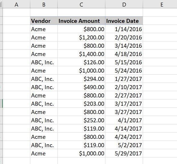
Practically speaking, we can eliminate the least and date values, because you’d be looking for a minimum value, and that’s not really the same thing as the last value. So that leaves us with the last record that matches the condition.
Simple, but not dynamic
We have two vendors, Acme and ABC, Inc., and let’s suppose we want to return the date and invoice amount for the last record in the data set for each company. You might think of VLOOKUP(), but that function returns the first matching value. There’s no way to force the function to find the last matching value.
If you control the data, you have an easy solution—reverse the records and use VLOOKUP(), which with a reversed data set, will find the last (first) record. The easiest way to reverse the record order is to populate a helper column with a set of consecutive numbers (Figure B).
Figure B
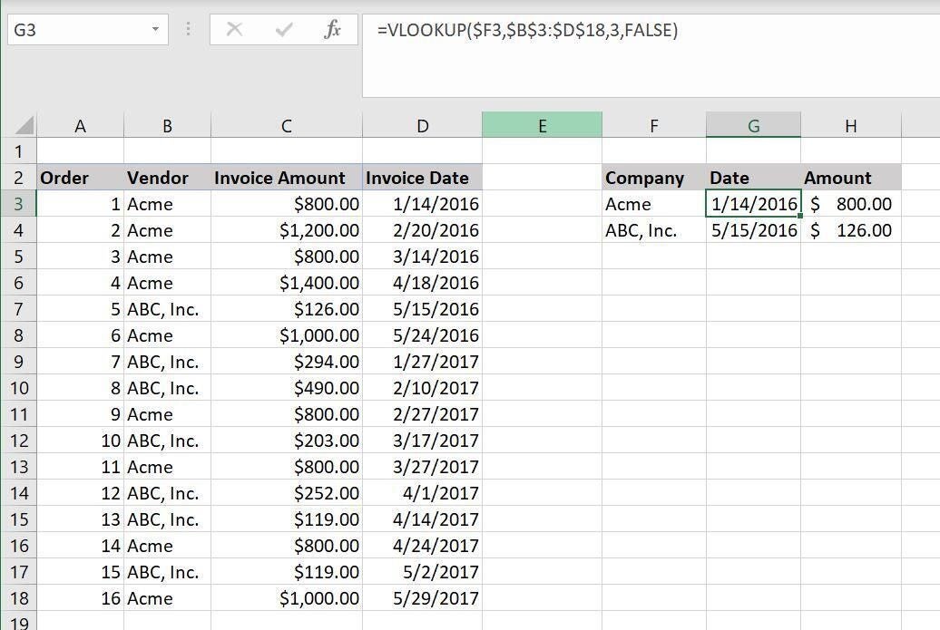
Next, let’s add the VLOOKUP() functions for returning the date and invoice (see Figure B). There are two lookup functions and the only difference between them is the return column:
G3: =VLOOKUP($F3,$B$3:$D$18,3,FALSE)
H3: =VLOOKUP($F3,$B$3:$D$18,2,FALSE)
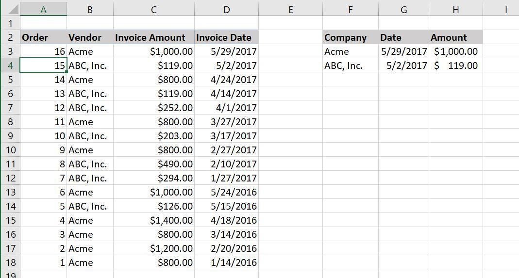
Copy the functions in row 3 to row 4. Right now, these functions return the first matching record for both companies. To get the last, reverse the data set by running a descending sort on the helper column you added. Figure C shows the results; now the VOOKUP() functions return the values for the “last” matching record. This is a simple solution, but it isn’t dynamic; you must remember to sort, which isn’t ideal.
Figure C
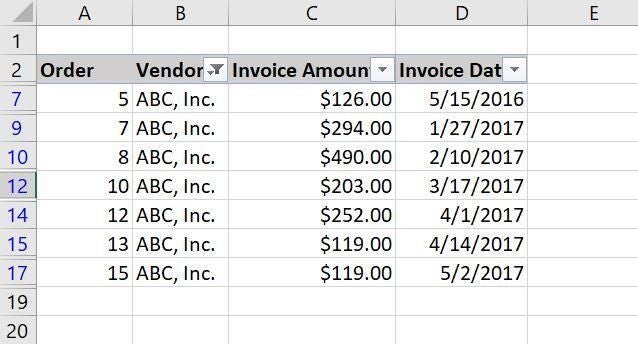
A simple filter will give you a quick visual (Figure D), if that’s all you need. To do so, click anywhere inside the data set and then click the Data tab. In the Sort & Filter group, click Filter. Then, use the dropdown list for the Vendor column and select only one company at a time.
Figure D
Dynamic
The VLOOKUP() and filter solutions are only partial solutions—having to remember to sort or getting just a visual clue isn’t enough. We can combine both partial solutions to create a good one that is dynamic and requires no extra action on your part other than filtering the data set. Using this solution, you can’t get both sets of data at the same time, but you might find it works better for you than the above solutions.
I’ve added a filtering row above the data set, and turned the data set into a Table object with a Totals row (Figure E). To create the Table, click any cell inside the data range, press Ctrl+t and click OK. To add the Totals row, click the contextual Table Design ribbon and check the Total Row option in the Table Style Options group. Finally, click inside the Order columns total cell—in the example sheet, that’s A20—and select Max from the dropdown. Doing so returns the maximum number in that column. Remember, the menu version doesn’t support the Table object.
Figure E
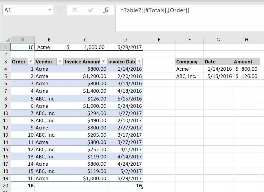
To create the filtering row, add the functions as follows:
A1: =Table2[[#Totals],[Order]]
B1: =VLOOKUP($A$1,Table2,2,FALSE)
C1: =VLOOKUP($A$1,Table2,3,FALSE)
D1: =VLOOKUP($A$1,Table2,4,FALSE)
As before, the VLOOKUP() function still finds the first matching value in the respective columns. The main difference is that the reference to the lookup table is a reference to Table2 (the Table we created). The expression in A1 references the value in the totals row for the Order column. That value is the result of a special SUBTOTAL() function that returns the maximum value in the filtered set.
In other words, the lookup value for the VLOOKUP() function is the value in A20—the largest value in the filtered set. Consequently, the function returns the corresponding values from that row.
With no filter in place, the filtering row always return the last row of values. Now let’s see what happens when we filter by company. To do so, choose only one company at a time from the Vendor columns dropdown. As you can see in Figure F, the filtered set for Acme returns the same values as a non-filtered set—that’s because the last row in the data set is an Acme record.
Figure F

Figure G shows the results of filtering for ABC, Inc. This time, the data changes to reflect the last record for that vendor.
Figure G
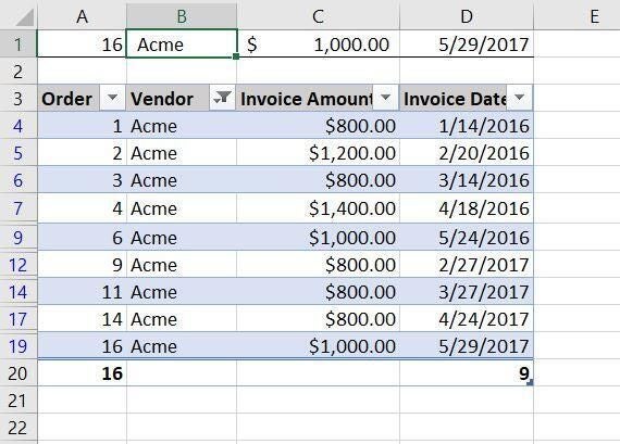
You still must filter the set to get the correct results in row A, but that’s much easier to remember than the sorting business from the earlier solution.