


Image: Wachiwit/Shutterstock
Must-read Windows coverage
- CrowdStrike Outage Disrupts Microsoft Systems Worldwide
- 10 Best Project Management Software for Windows in 2024
- Windows 10 Extended Security Updates Promised for Small Businesses and Home Users
- Securing Windows Policy
The article How to do more advanced averaging in Excel reviews Microsoft Excel’s many averaging functions. The focus is how the functions evaluate zero and Boolean values and empty string values. These functions won’t always be adequate, though. In fact, sometimes you’ll need an expression that doesn’t use any averaging functions at all. In this article, we’ll look at some unique averaging solutions.
SEE: 69 Excel tips every user should master (TechRepublic)
I’m using Microsoft 365 on a Windows 10 64-bit system, but you can use earlier versions. You can download the demonstration .xlsx and .xls file, or work with your own data. All functions are supported by the browser.
A quick review of averaging in Excel
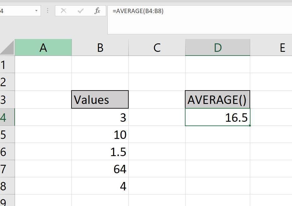
Just in case you’re not familiar with the AVERAGE() function, we’ll start with a quick review of this function. As you might expect, this function adds the referenced values and then divides that total by the number of values. You can reference cells, a range, and even literal values. It’s important to remember how this function deals with non-traditional values:
- Text is ignored
- Logical, or Boolean, values TRUE and FALSE are ignored.
- Empty cells are ignored.
- If the function references an error value, it returns an error.
As you can see in Figure A, AVERAGE() returns the average value of a simple data set. The resulting average is the same as if you totaled and divided: =SUM(B4:B8)/5. We’ll continue to work with this data set while we complicate things a bit.
Figure A
How to average only high and low in Excel
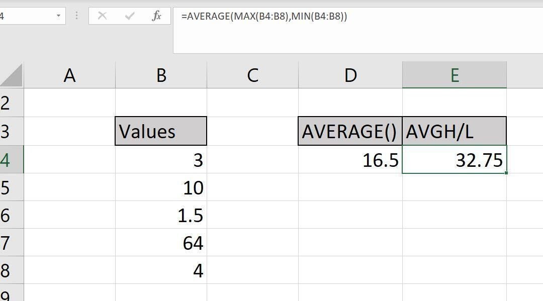
Averaging the highest and lowest values in a data set seems like an obscure requirement, but I’m including it so you can see the way AVERAGE() can work with other functions. For this solution, we’ll combine AVERAGE(), MAX() and MIN(). Figure B shows the results of the function
=AVERAGE(MAX(B4:B8),MIN(B4:B8))
and returns the value 32.75, the same value the expression (1.5+64)/2 returns.
Figure B
It’s easy to determine how this function works, but let’s evaluate it using the example data set:
=AVERAGE(MAX(B4:B8),MIN(B4:B8))
=AVERAGE(64,1.5)
32.75
This function is simple, but sometimes you won’t want to eliminate specific values, but rather, a percentage of values. That’s what we’ll tackle next.
How to get a trimmed mean in Excel
You probably know that mean is an average. For the most part, the only difference is the term: Mathematicians use average and statisticians use mean. However, not every mean is an average because there are different kinds of means. The term arithmetic mean and average are synonymous, though.
SEE: Windows 10: Lists of vocal commands for speech recognition and dictation (free PDF) (TechRepublic)
With that discussion to fill in a few gaps, it’s time to introduce Excel’s TRIMMEAN() function, which removes a designated percentage of the largest and smallest values, otherwise known as a trimmed mean. This happens when outliers are extreme and skew the results—by removing the values, the average is a bit more realistic.
TRIMMEAN() removes a percentage from both ends, so sometimes it will end up being only the largest and smallest; sometimes it will remove two or more values from both ends. It’s unlikely that the average user will ever need this function, but I’m including it to be comprehensive.
This function uses the form
TRIMMEAN(range,percentage)
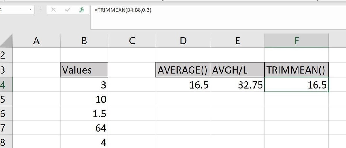
where range references the evaluated values and percentage denotes how many values to remove from both ends. You can enter percentage using one of two formats: 0.2 or 20%. Our small data set returns the same value for both AVERAGE() and TRIMMEAN(), as shown in Figure C. In this case, the percentage, 0.2 returns 1 value to be removed (5 values divided by 20% equals 1). That value is split between the two ends, highest and lowest, and of course, you can’t remove half a value, so it removes none. The two results will remain the same until you change percentage to 40% (0.4).
Figure C
It’s a bit unfortunate because TRIMMEAN() doesn’t provide a more realistic result with our data set, as you just saw. Let’s look at an expression that will.
How to exclude high and low in an average in Excel
It’s common to eliminate the highest and lowest values, or outliers, when averaging. Teachers and statisticians do so frequently. What we’re doing is similar to the function in the previous section, but TRIMMEAN() removes a percentage; in this example, we want to remove only the highest and lowest value, not a percentage of values.
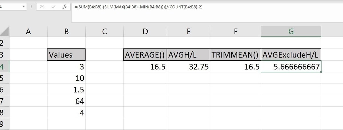
Although the expression shown in Figure D
=(SUM(B4:B8)-(SUM(MAX(B4:B8)+MIN(B4:B8))))/(COUNT(B4:B8)-2)
is long, it isn’t complicated; it just has a lot of parts. In a nutshell, it returns the same thing as SUM(3,10,4)/3. The values evaluated exclude 1.5 and 64.
Figure D
Let’s evaluate this expression using our data set:
=(SUM(B4:B8)-(SUM(MAX(B4:B8)+MIN(B4:B8))))/(COUNT(B4:B8)-2)
=(82.5)-(64+1.5)/(5-2)
=17/3
5.666666667
I’m not convinced that there isn’t a shorter expression, but the logic in this one works. From the sum of the entire data set, you subtract the sum of the two outliers (64 + 1.5). Then, you divide that total, 17, by 3, because there are only three values evaluated. You will always subtract 2 from the total number of values because you remove only two values from the data set.
These averaging solutions are a tad severe; you won’t always have such rigid restrictions. When you do, with a little know-how, you can get the job done.