Power BI is Microsoft’s standard data visualization tool. It is available for free as a web service or as part of one of the business editions of Office 365. However, while it is generally available to just about everyone, it is not used as often as it might be. That is a problem, because in the age of big data and the Internet of Things (IoT), data visualization plays a vital role in business communication and decision making.
One of the simplest ways to take advantage of Power BI’s data visualization abilities is to link it with an Excel workbook–it is the way most business users will employ the Power BI tool. But there are some key tips to keep in mind before you attempt to link your Excel workbook. This quick tutorial will show how to prepare your workbook for Power BI.
SEE: Microsoft Power BI: The smart person’s guide
Flatten your data
For Excel power users, this may come as a bit of a shock, but workbooks destined to be linked to Power BI for its data visualization tools must be restricted to flat data. That means no matrix views and especially no pivot tables.
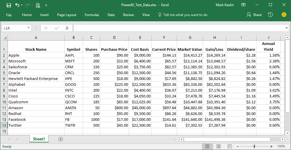
Take a look at the example Excel workbook shown in Figure A. It is a list of stocks and some common data points typically associated with stocks: shares, prices, gain/loss, etc. Notice that there are no summed columns or rows, just column headings.
Figure A

In general, an Excel workbook like this one would have conditional formatting, summed columns, and so on. If you have a workbook you want to link to Power BI with those kinds of analysis already embedded, you will have to deconstruct it until you get down to a pristine list of flat data.
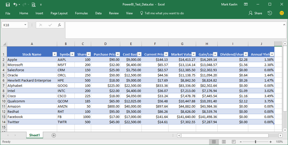
The next step is to convert your flat data into the standard Excel table format. The easiest way to do this is by highlighting the data in your workbook and pressing Ctrl + T. Or, if you prefer, you can click the Format As Table icon in the Ribbon of the Home Tab. Make sure the box that indicates your data has column headers is checked. This procedure will allow you to convert your flat data into a standard Excel table, as shown in Figure B.
Figure B

This last step is optional, but it is recommended as a way to reduce confusion in the future. You should name your table something descriptive that you will recognize and understand later. Highlight the cells of the table, click the table name box and give it a new descriptive name. I named my workbook ITStocksTestData. Note: you can’t use spaces in an Excel table name.
SEE: Microsoft Teams: The smart person’s guide
Preparation is key
Now your Excel workbook is ready to be linked to Power BI. If you do not prepare your workbook in this way Power BI will just ignore it, so this process can’t be avoided.
The Power BI how-to series
This tutorial is first in a series of tips and tricks that will help you reap the benefits of Power BI and data visualization. The series also includes these topics:
- How to create your first Power BI dashboard
- How to harness OneDrive to keep your Power BI dashboard fresh
- How to share your Power BI dashboards and reports
The entire series is available as a PDF ebook.
Also read…
- Microsoft wants to bring better data visualization to your enterprise
- Microsoft’s Satya Nadella thinks these four technologies will reshape IT
- Hiring kit: Microsoft Power BI developer (TechPro Research)
- Mobile analytics: 10 great apps to visualize big data on the go
Your thoughts
Have you tried using Power BI? Did you have trouble getting Excel to work with it? Share your thoughts and opinions with your peers at TechRepublic in the discussion thread below.
