How to find duplicates in Google Sheets

Google Sheets offers several ways to compare, identify, and remove duplicate data in cells and rows. These features can help you find cells where data matches, then signal that a difference exists text. Sheets lets you quickly remove rows that contain duplicate data.

Each of the following methods lets you detect and deal with duplicate Google Sheet cell content. You can combine the first two methods as desired, so you could add a cell that signals that cells are the same and sort your sheet, too. However, the third option (which removes duplicates) deletes data, so use it with care.

In every case, to detect duplicates, you’ll want to open the Google Sheet you want to review. You’ll need edit permissions to use the features below. And, while you can add formulas for cell comparison in the Google Sheets mobile apps, you will need to use Google Sheets in a desktop-class browser (such as Chrome) to sort data or use the remove duplicates feature.

SEE: Google Sheets: Tips every user should master (TechRepublic)

How to sort rows of data by columns you choose in Google Sheets

A sort helps make duplicate data in Google Sheet rows easier to review, since it places rows in alphabetical (or reverse alphabetical) order. You may sort by more than one column. For example, you might sort by a Last Name column, then sort by a First Name column to place rows of data where the last and first name match next to each other. When sorting to detect duplicate customer data, for example, you might also sort by phone numbers or street addresses. You may sort a Google Sheet by any column you choose.

1. Select the cells you want to sort. One way to do this is to click or tap in the upper left cell, then drag to the lower right cell in the range.
2. Choose Data | Sort Range. Google Sheets will display several sort options.
3. Configure your sort options (Figure A).

Figure A

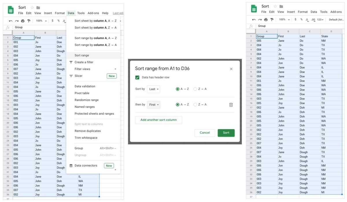
4. First, select the checkbox If Your Range Of Data Has A Header Row. This will exclude this row from the sort.
5. From the Sort By dropdown menu, select a column to sort. You may change the sort order from the default (A to Z) to reverse alphabetical (Z to A), if desired.
6. For a secondary sort, you may select Add Another Sort Column, then choose the column and sort options. Repeat this step for as many sort columns as desired.

After sorting rows of data by columns, you may manually review data, then select and delete duplicates as needed.

SEE: 10 free alternatives to Microsoft Word and Excel (free PDF) (TechRepublic)

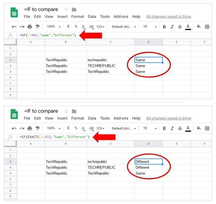
How to compare cells in Google Sheets

In some cases, it may be useful to compare the contents of cells, then display a word in another cell that indicates whether the contents are the same or different. In Google Sheets, the =IF formula provides a way to compare contents, then return a different result when the comparison is true than when it is false. Additionally, unlike conditional formatting, which may be difficult for some people to see, an =IF comparison puts text in a cell to convey the comparison status.

1. In a cell outside of your data range (typically in the same row as your data), enter the following formula:

=IF(C3=B3,"Same","Different")

2. Replace the cell numbers in the example (e.g., C3 and B3) with the two cell references you wish to compare.

3. You may adjust the text. The first term above (i.e., “Same”) displays when the condition is true. The second term above (i.e., “Different”) displays when the condition is false.

Note: With this formula, the system does not differentiate capitalization, so it will consider “TechRepublic” and “TECHREPUBLIC” and “techrepublic” all as equal and therefore duplicate content. For a strict comparison, use an additional command:

=IF(EXACT(C3,B3), "Same," "Different")

This formula requires that the contents of the two cells be an exact match (Figure B).

Figure B

Of course, logic statements can expand if you need to compare more than two cells. For example, you can compare the contents of cells B3, C3, and D3 with the following formula:

=IF((AND(C3=B3,D3=B3)),"Three same","Not all three are the same") 

As with a sort, the contents of these comparison cells help you identify duplicate data.

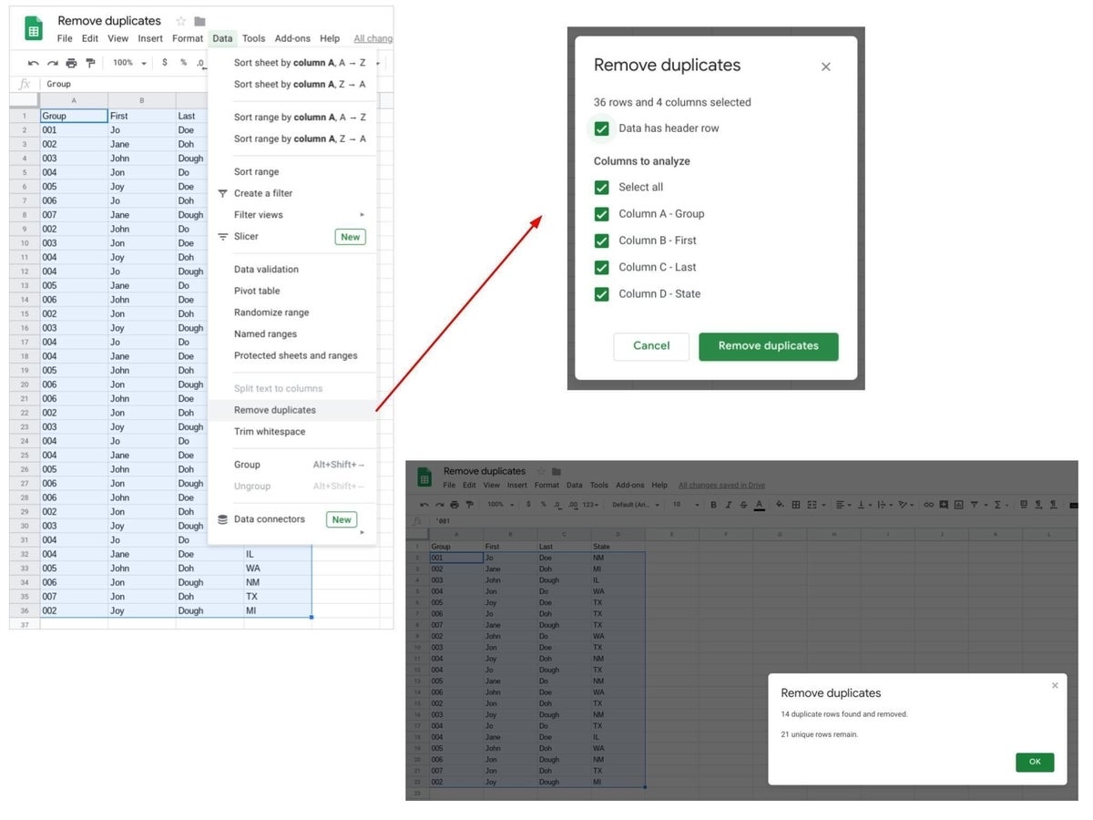
How to remove duplicates in Google Sheets

Google Sheets includes a built-in option to remove duplicate rows of data within a selected range. When the system identifies rows with the same data, it retains one and deletes all other duplicates. Since the command deletes data, you may want to name your Sheet With File | Version History | Name Current Version before you remove duplicates. A named version allows you to refer to the Sheet contents prior to duplicate deletion.

1. Select a range of cells to compare.
2. Choose Data | Remove Duplicates. The system will remove any duplicate rows found. Google Sheets will display how many duplicate rows were removed, as well as how many unique rows remain (Figure C).

Figure C