How to split a column using an IF() function in Excel

We all inherit Microsoft Excel sheets that don’t suit our working routine. If it’s a simple tracking sheet of some sort, you can usually change things to suit your working needs.

For instance, it’s not uncommon to work in a sheet that follows traditional database design rather than a financial sheet structure. When this happens, you can usually revamp the structure by employing a few expressions instead of creating the new structure from scratch. In this article, I’ll use two IF() functions to split a simple “database” sheet into multiple columns, based on a value in another column.

Disclosure: TechRepublic may earn a commission from some of the products featured on this page. TechRepublic and the author were not compensated for this independent review.

I’m using (desktop) Office 365, but you can work with earlier versions. For your convenience, you can download the demonstration .xlsx file, but you can also work with your own data. The expressions will work in the browser edition.

Why you might use the IF() function

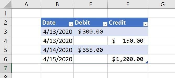
In database fashion, a lot of data is defined by type. That way, you only need one field for the actual value. You can do this with Excel, too, as shown in Figure A. This simplified table uses only one value field and defines each value as either a debit or a credit. In Excel, you might also see this as two value columns, one for debits and one for credits, and no transaction type field because that’s identified by each column header.

Figure A

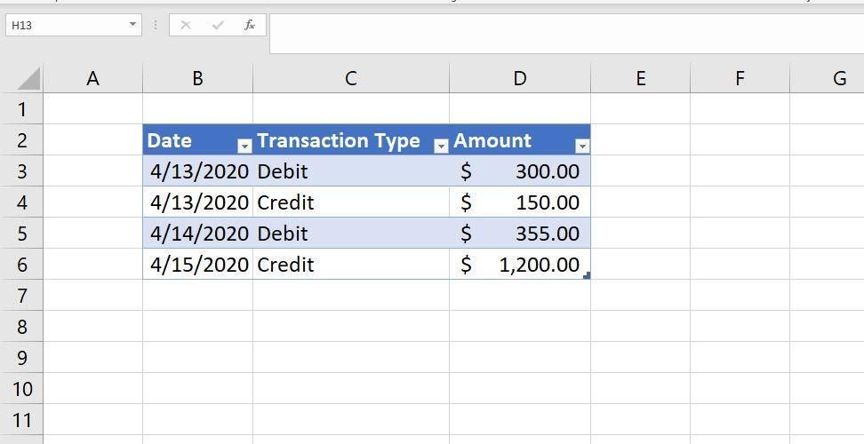
If you inherit a sheet that resembles the one in Figure A, but you want a more traditional sheet where the two transaction types are in different columns, you’re not stuck. You might try Text to Columns first, but in this case that feature won’t work because it works with a single column. You can’t use it to split values based on a conditional value in a second column. Instead, we’ll use two IF() functions, one for debit and one for credit.

The IF() function uses the following form:

IF(condition,true,false)

where condition is a value or expression that equates to true or false and the true and false arguments identify what happens when condition is true or false, respectively. Now, let’s put this function to use.

How to make the debit expression

There are several string functions for delimiting strings, but we need a conditional expression. For that reason, we’ll use two different IF() expressions: One that returns debit value and one that returns credit values.

Let’s start with the debit values. First, create a new column by entering Debit in cell E2. If you’re working with a Table object (as I am), Excel will automatically extend the Table. In E3, enter the following expression:

=IF(C3=”Debit”,D3,””)

Copy the expression to the remainder of the column. Figure B shows the two debit values in column E.

Figure B

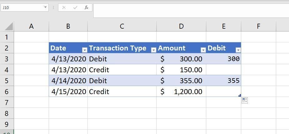
At this point, column E contains only existing debit values from column D. If the value in column C equals “Debit,” the function returns the true argument, which is the corresponding value in column D. Otherwise, the function returns a blank string (“”). As you can see, column E contains only two values, the values where the corresponding text in column C is Debit. Now, we need a column for credits.

How to make the credit expression

Now that you’ve split out the debit values with an IF() expression, you can probably do the credit values on your own. In F2, enter Credit, and again the Table object will extend the Table. We’ll use the same basic function, but this time, we’ll use Credit as the condition:

=IF(C3=”Credit”,D3,””)

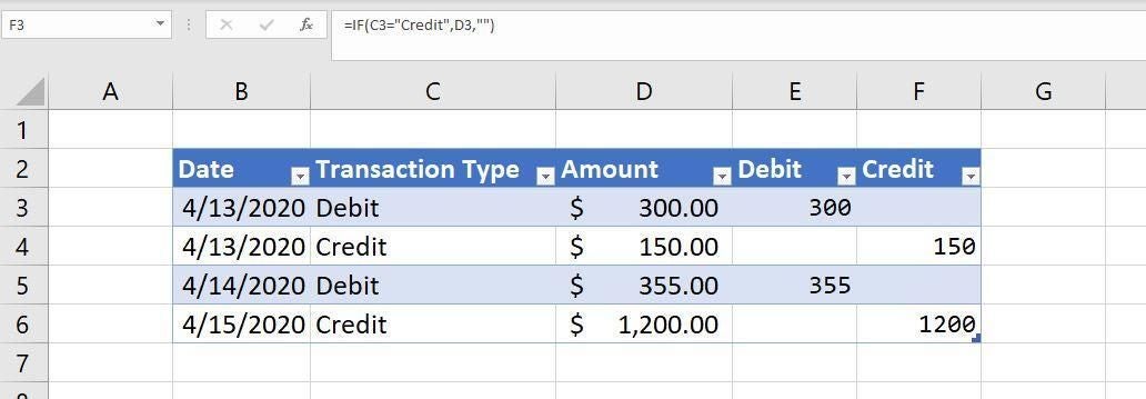
As you can see in Figure C, we now have two columns: Column E displays debit values, and column F displays credit values. But we’re not done yet.

Figure C

The difference between formulas and values

Right now, it looks like we’re done, but we really aren’t. The values in columns E and F are the results of two IF() functions, and we need literal values.The IF() functions are only a temporary means of getting the existing values into the structure we want to use going forward.

To convert the formulas, do the following:

1. Select E3:F6 (the range containing the IF() functions).
2. In the Clipboard group (on the Home tab), click Copy.
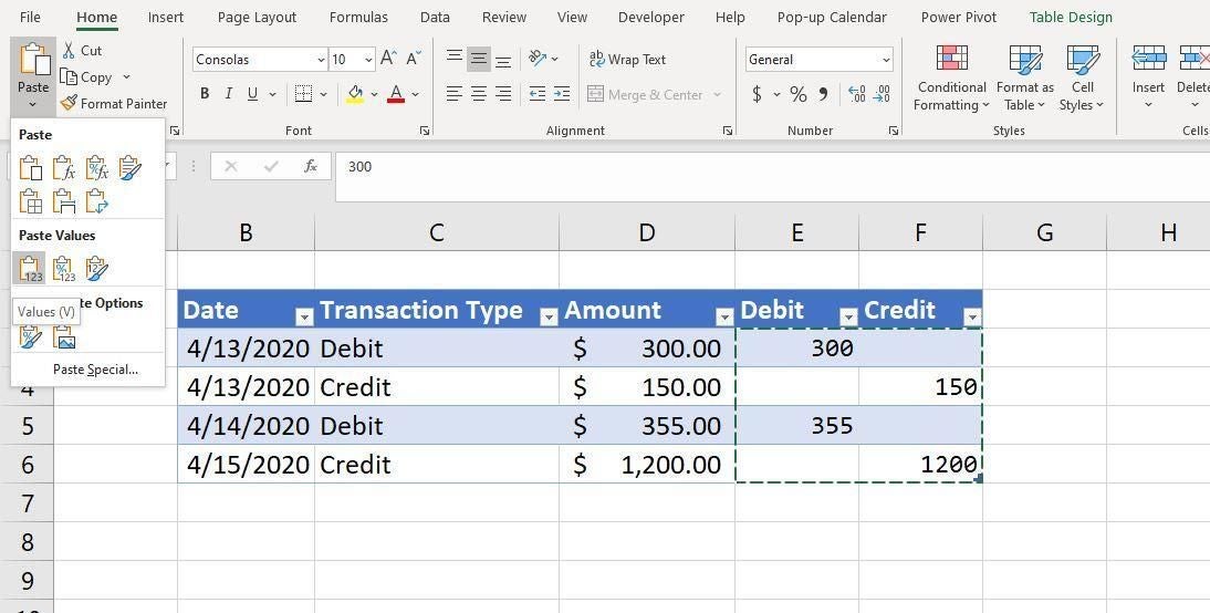
3. In the same group, click the Paste dropdown and choose Values (the first option) in the Paste Values section (Figure D). After doing so, the values in columns E and F are now literal values—the IF() functions are gone.

Figure D

How to clean up your columns

Now that you have the original values split into columns, you can clean things up a bit. First, you’ll want to format the new values in columns E and F. In this case, apply the Currency format. Second, you should delete or hide columns C and D—they are no longer needed. Figure E shows the finished results. Now, users can enter debits and credits in columns E and F, respectively.

Figure E