


Illustration: Lisa Hornung
Must-read Windows coverage
- CrowdStrike Outage Disrupts Microsoft Systems Worldwide
- 10 Best Project Management Software for Windows in 2024
- Windows 10 Extended Security Updates Promised for Small Businesses and Home Users
- Securing Windows Policy
Styles are a Microsoft Word feature, right? You might be surprised to learn that Microsoft Excel uses styles too, although the nature of the data doesn’t require the same kind of robust options. Excel styles are easier to use than Word’s. If you’re not using them because you think they’re complicated, you might want to reconsider. In this article, I’ll introduce you to Excel styles and show you how to use them to use more efficiently in Excel.
I’m using (desktop) Office 365 but you can use an earlier version. You can work with your own data or download the demonstration .xls file. Styles are available in the browser edition.
What’s a Microsoft Excel style?
If you don’t work with styles, you might be wondering what’s so special about them. The easy answer is, they help you work more efficiently. A style is a collection of formats that you can apply simultaneously. For instance, you might want all input cells to have a green background with white font. By using a style, you can apply both formats at the same time. Now, that doesn’t sound like a big deal, but there’s more. If you decide to change the format for input cells, you don’t have to change all those cells individually. You simply change the style and all input cells update automatically—now that’s working efficiently.
Styles in Microsoft Excel
Styles aren’t as obvious in Excel (and other Office 365 apps) as they are in Word. On the Home tab, you’ll find styles in the Styles group, Format a Table, and Cell Styles. We’re going to work with the Cell Styles option. As you can see in Figure A, the dropdown offers several built-in cell styles.
Figure A
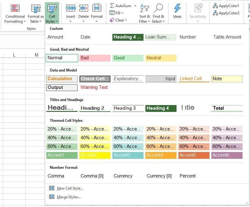
Whether or not you realize it, you’re using a style called Normal—that’s the sparse formatting you see when you enter data in a new sheet. Toward the bottom of the gallery (Figure A) you’ll see Comma, Comma[0], Currency, and so on. You’re also already using these styles when you choose a from from the dropdown in the Number group.
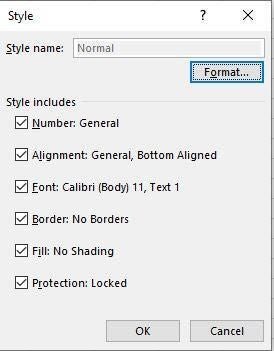
To quickly assess a style’s formatting, without applying it, right-click it in the gallery and choose Modify. The resulting dialog shown in Figure B shows Normal’s formats. Not all format types will be present, as in this one.
Figure B
Working with styles in Excel
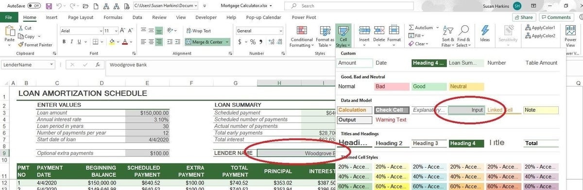
If you’re working with an existing workbook, chances are someone used a style or two. For example, let’s suppose you open Excel’s Mortgage Calculator.xlsx template. You’ll see data and some formatting that makes the sheet more readable. Select a formatted cell and then click the Cell Styles dropdown. In Figure C, you see that cell I9 has the Input style applied. You can tell by the heavy border around the current style (in the gallery).
Figure C
This bit is important: If you see formatting but Normal is selected in the Styles gallery, you know that you’re seeing direct formatting; that format was applied manually. Direct, or one-off, formatting is fine, but when you start mixing it with styles too much, things can get confusing. It’s better in the long run to modify the style than to manually apply more formatting to a cell that has an applied style.
Let’s see what happens to cell I9 when we modify the Input style:
- Click the Cell Styles dropdown, and right-click Input.
- Select Modify.
- In the resulting dialog, click Format.
- Click the Fill tab and choose a different color, say a light orange.
- Click OK twice.
As you can see in Figure D, cell I9, now has that light orange background. Were you expecting all of the gray cells, E3:E9 to change fill color? (I was.) The explanation is simple: Only I9 is using the Input style. The gray cells in column E use other styles, such as Amount, Percent, and so on. If you check these styles, you’ll find that they do not include a fill color. Therefore, the gray fill color is a direct format. The advantage, at this point, is knowing the underlying styles so you can modify formatting with minimal confusion and effort. Remember, changing a style is preferred to lots of direct formatting.
Figure D
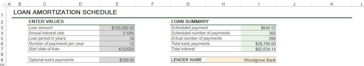
Now, let’s make a more drastic change. Let’s suppose that you want to add bold to the italicized cells in columns E and G and change the font color to dark green. Now, you could use direct formatting on one of those cells and then use the Format Painter, but modifying the applied style is quicker and guarantees consistency in the future. Let’s try that.
First, check one of the cells to see what style is applied. (I showed you how to do that earlier. In this case, the style is Explanatory. With the gallery open, continue as follows:
- Right-click the Explanatory style (in the gallery).
- In the resulting dialog, click the Format tab.
- Click the Font tab and change the Font Style to Bold Italic.
- From the Color dropdown, choose dark green (Figure E).
- Click OK twice.
Figure E
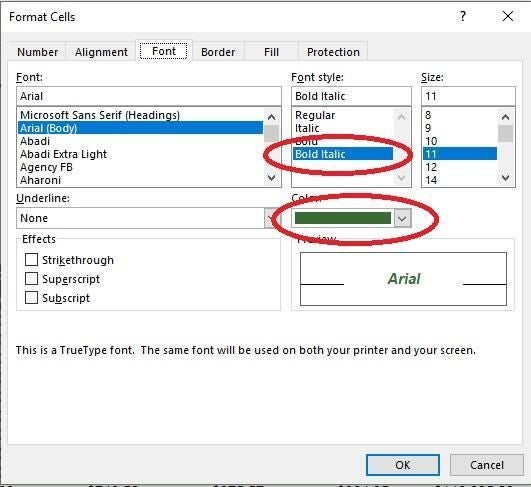
Figure F shows the updated cells. It only took a few clicks to change all those cells.
Figure F
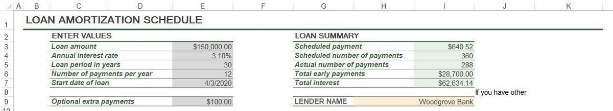
We updated the Explanatory style, changing the formatting for several cells at once. It’s important to remember that if you have other cells with the same style, they will update, too. In most cases, that’s what you’ll want. If not, you might need to create a new style. Use the Duplicate option instead of choosing Modify (in the gallery), then name the new style and make changes. It’s quicker than starting from scratch.
One more thing
Cell styles reflect the theme that’s applied to the entire workbook file. When you change one theme to another, cell styles change accordingly.
Excel cell styles are easy to implement. Knowing they exist and how to determine what’s in use and how to modify a style are the keys to using them efficiently.