How to turn an Excel sheet into graph paper

This past week, I started mapping out new flowerbeds on graph paper. Now, graph paper’s cheap, but making changes takes time and sometimes you just have to start over. Unfortunately, I don’t have specialized software aimed at garden design, so I thought about what I do have – I have Excel! With just a little work, I turned an Excel sheet into a modifiable piece of graph paper.

The trick is to square up the cells. The gauge is less important. Like graph paper, a cell can equal anything you want. The hard part is getting the width and height settings to produce a square because there’s no easy way to match a cell’s height and width settings. You can’t just set the row height and column width to the same value because:

• Excel measures row height in points.
• Excel considers the current font when calculating column width; a column width of 5 means that the column will display 5 digits, using Normal style.

You could spend a lot of time tweaking the height and width and you could even try holding a ruler up to your screen, but there’s an easier way: Format an AutoShape as a square and use it as a guide. First, you need to insert and format an AutoShape as follows:

1. From the Drawing toolbar, choose Basic Shapes from the AutoShapes drop-down list.
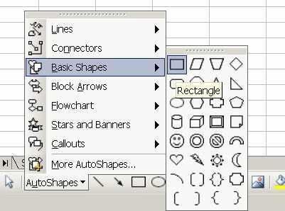
2. Double-click the rectangle (the first shape in the first row) and Excel will insert a rectangle into the current sheet.
3. Right-click the rectangle and choose Format AutoShape.
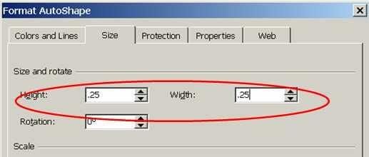
4. Click the Size tab.
5. In the Size And Rotate section, enter .25″ for both the Height and Width to create a square. If you want a larger square, enter a larger value for both measurements.
6. Click the Properties tab, select the Don’t Move Or Size With Cells option, and click OK.
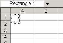
7. Back in the sheet, move the rectangle (it’s a rectangle object, shaped as a square), to the top-left corner, just over cell A1.

Now, use any method you like to resize both the height and width. Perhaps the easiest way is to drag the header and row cells to the appropriate position as follows:

1. Select the entire worksheet (or the area you want to resemble graph paper). To select the entire sheet, click the sheet selector – that’s the cell that intersects the row and column headers (in the top-left corner).
2. Hover the mouse over the right border of column A’s header cell.
3. When the cursor turns into a double-arrow, drag the border until it’s flush with the rectangle’s right border. Excel will resize the width of all the selected columns, not just column A.
4. To resize the height, adjust the bottom border of row 1 until it’s flush with the bottom of the rectangle. Again, Excel will adjust all the selected rows.

At this point, you have a sheet full of .25-inch cells. Move the AutoShape rectangle at cell A1 or delete it – you’re done with it. If the cells are still a bit too large, set the Zoom property to 50%. Then, start adding the appropriate components by formatting cells and adding AutoShapes. Be sure to add a legend to identify all those components.

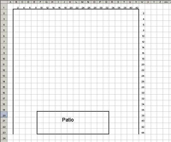
As you change your mind, it’s easy to reformat cells and delete objects. No more erasing, no more starting over!