


Analyzing data often means spending more time getting and cleaning up data than analyzing it. If that describes you, definitely review Excel 2016’s Power Query (or Get & Transform). Using Power Query, you can load data from several different sources, including the active workbook. Once data is in Power Query, you can analyze and manipulate that data quickly using specialized tools. If you think the only way to get the results you need is to use complex formulas or even VBA code, take a step back and think, Can I do this in Power Query instead? Often, the answer will be yes.
In this short introduction to Power Query, I’ll show you a problem that requires some fancy hoop-jumping to manage, unless you use Power Query. Specifically, I’ll show you how to create a database-style structure by separating multiple values stored in the same column into individual rows–one row for each value. It’s a common problem and not easily solved in Excel without specialized knowledge.
More about Software
- Software Installation Policy
- Five Methods to Insert a Checkmark Into Microsoft Office Products
- How to Hide and Handle Zero Values in an Excel Chart
- How to Use Section Breaks to Control Formatting in Word
I’m using Office 365’s Excel 2016 (desktop) on a Windows 10 64-bit system. Power Query, otherwise known as Get & Transform, is available in earlier ribbon versions, but you need to install it as an add-in. There’s no comparable tool in earlier menu versions. You can use your own data or download the demonstration .xlsx file.
What’s a multi-value field
If you’re familiar with database technology, you know that one of the most important normalization rules is that each field should store the smallest possible autonomous value. Many databases and especially spreadsheets break this rule, much to their users’ sorrow. Figure A shows a simple data set that breaks this rule.
SEE: Software Usage Policy (Tech Pro Research)
Figure A
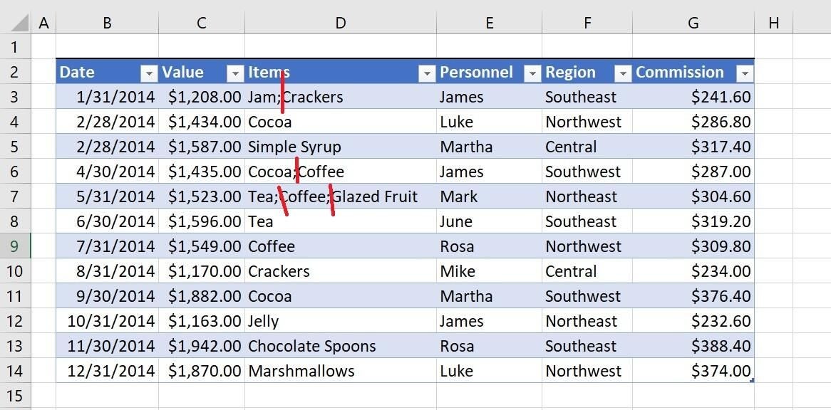
A multi-value field stores one or more values.
As you can see, three records (rows 3, 6, and 7) have more than one value in the Items column. It makes sense, but only at first. It won’t take long to realize that you can’t easily analyze or manipulate by the subsequent values. For instance, how would you count the number of items represented in this data set? (There’s 16).
If you stored this data in a relational database, you’d have at least two tables: One for each order with a primary key that uniquely identified each record (order) and a second that stored each product as a single record. Then, you’d use a query to pull those records together–one record for each product using a primary/foreign key to identify, which products go with which order. Using this structure, you can easily sort, group, and even analyze your data by the Items values without jumping through any hoops.
That’s what we’re after with the simple sheet shown in Figure A. We want a record for each value in the Items column. Specifically, instead of 12 records, we want 16, and we want a way to group the products for each order. Can you see the problem? Trying to do this manually would be worse than tedious. Serious developers would turn to VBA, but what if you don’t have that skill? Thanks to Power Query, even casual users can create 16 records from 12 in only a few minutes:
- First, we’ll load the data into Power Query.
- Then, we’ll add an index column, so you can visually see which products belong to the same order.
- Next, we’ll create the new rows using a delimiter query. A delimiter is a constant character that separates values.
It’s quick, and it’s easy.
Load data into Power Query
I mentioned earlier that you can load data from lots of sources; I recommend that you explore the many options (Figure B) on your own. For now, we’re going to load data from a Table object already in Excel. If your data is a normal range, you must convert it to a Table object; if you don’t, Excel forces you to do so when you engage the feature.
Figure B
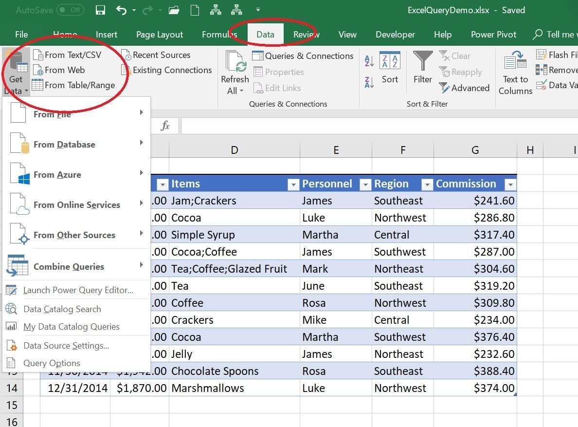
Power Query can retrieve data from many sources.
To convert a data set into a Table object, click anywhere inside the data set, click the Insert tab, choose Table from the Tables group, specify whether the data set has a header row, and click OK.
To load the Table object into Power Query, do the following:
- Click anywhere inside the Table.
- Click the Data tab.
- In the Get & Transform Data group, click From Table/Range. (If the data isn’t a Table, Excel will run you through the steps necessary to convert the data into one.)
- Excel will launch the Query Editor (Figure C). Each column header identifies its data type for easy visual confirmation.
Figure C
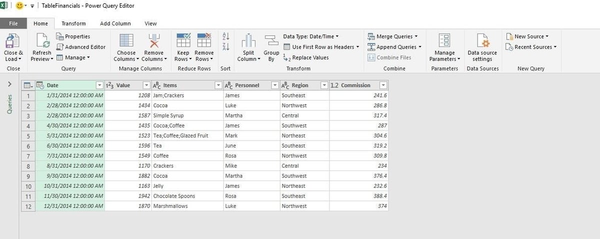
The Query Editor offers many tools for manipulating and analyzing data.
Add an index column
This next step isn’t necessary, but it adds a powerful visual “Ohhhhh!” moment that I think you’ll appreciate. We’ll add a unique value to each row–remember, right now, each row represents a single order, but some of the orders comprise multiple products.
To add an index column:
- Click the query menu (the sheet icon at the intersection of the header rows).
- From this menu, choose Add Index Column, and then select From 1 from the resulting submenu (Figure D).
Figure D

Select a seed for the index column.
As you can see in Figure E, each record has a unique value. The series starts with one and is consecutive. We have 12 order records.
Figure E
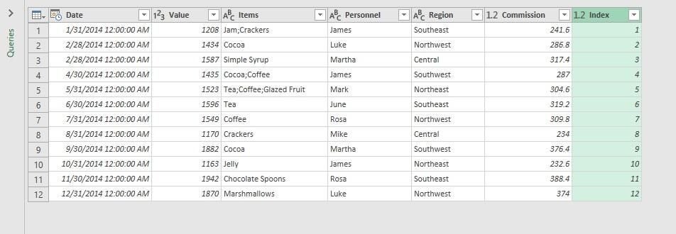
Add an index column to the data set.
A little magic
Now we’re ready to work a little magic–or rather, let Excel work some magic. Remember, we want a single row for each Items value, not each record. The solution is easy:
- Select the Items row (click the header cell).
- Click the Split Column option in the Transform group, and choose By Delimiter from the resulting dropdown list.
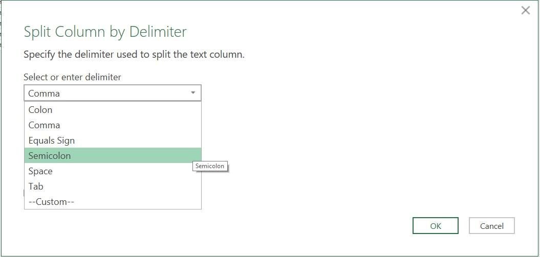
- The resulting dialog prompts you to identify the delimiter; in this case, it’s the semi-colon (;) (Figure F), so select Semicolon from the dropdown list. Retain the default option, Each occurrence of the delimiter, but don’t click OK yet.
- Click Advance options.
- In the Split into section, select Rows (Figure G) and click OK.
Figure F
The query returns a single row for each value in the Items column.
Figure G
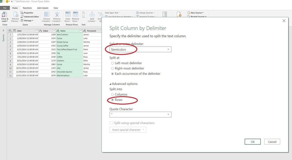
Specify a row split.
As you can see in Figure H, each item moved to a row of its own, along with the order information: date, Value, and so on. The index column helps you discern, which products belong to the same order. The index values still identify the original 12 orders, but there’s more than one row for order 1, 4, and 5, which indicates those orders have multiple items. You can put your hoop away–no jumping required. This is where you say, “Ohhhhhhh!”
Figure H
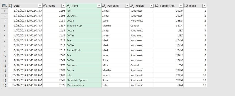
Power Query separates each item value into a row of its own.
When you close Power Query, Excel prompts you to keep or discard the query. If you want to work with the data, choose Keep. Excel copies the results of the query into a new sheet.
Send me your question about Office
I answer readers’ questions when I can, but there’s no guarantee. Don’t send files unless requested; initial requests for help that arrive with attached files will be deleted unread. You can send screenshots of your data to help clarify your question. When contacting me, be as specific as possible. For example, “Please troubleshoot my workbook and fix what’s wrong” probably won’t get a response, but “Can you tell me why this formula isn’t returning the expected results?” might. Please mention the app and version that you’re using. I’m not reimbursed by TechRepublic for my time or expertise when helping readers, nor do I ask for a fee from readers I help. You can contact me at susansalesharkins@gmail.com.
See also
- Three running total expressions for Excel (TechRepublic)
- Five tips for using Outlook 2016’s AutoComplete list efficiently (TechRepublic)
- How to use VBA to select an Excel range (TechRepublic)
- Excel errors: How Microsoft’s spreadsheet may be hazardous to your health (ZDNet)
- Office Q&A: How to handle end-of-sentence spacing in Microsoft Word (TechRepublic)
- AI helps Google Sheets grok your plain-English commands (CNET)