


The article, How to use a border to discern groups more easily in Microsoft Excel, shows you how to use a conditional formatting rule to apply a red border between groups in an Excel sheet. It’s not as effective as you might like because the border is so thin. In this article, we’ll use a conditional format to apply a fill color to each row in the same group. This technique does come with a limitation that I’ll explain at the end of the article.
SEE: Software Installation Policy (TechRepublic Premium)
Must-read Windows coverage
- CrowdStrike Outage Disrupts Microsoft Systems Worldwide
- 10 Best Project Management Software for Windows in 2024
- Windows 10 Extended Security Updates Promised for Small Businesses and Home Users
- Securing Windows Policy
I’m using Microsoft 365 on a Windows 10 64-bit system, but you can use an earlier version. For your convenience, you can download the demonstration .xlsx and .xls files. Excel for the web supports rules in the conditional format feature, but you are limited to the formats you can choose.
How to group the data in Excel
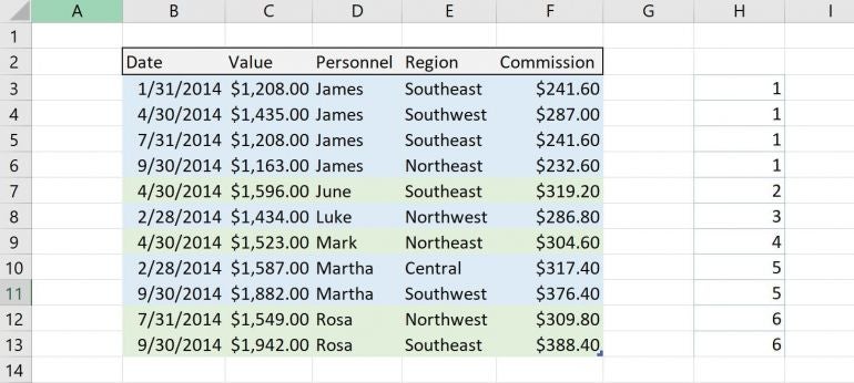
Because we’re formatting groups, the data must be grouped before you begin. If your data is already sorted by the grouping values, then you can skip this step. The demonstration file isn’t sorted yet, so let’s get started. We want to group by Personnel values. Click inside any cell in the Personnel column. In the Editing group on the Home tab, choose A to Z from the Sort & Filter dropdown. The result is that the sales and commissions for each personnel are grouped (Figure A).
Figure A
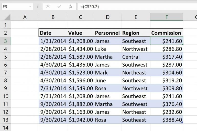
If the data is already formatted with colored bars, delete the format. This is easily accomplished by selecting the data, in this case, B3:F13 and choosing No Fill from the Fill Color dropdown in the Font group on the Home table. If, however, you’re working with a Table object, choose None in the gallery in the Table Styles group on the contextual Table Design tab.
Grouping the data by sorting and removing existing formats is necessary for this technique to work. Now, let’s move on to the helper function.
How to create a helper function in Excel
Once the data is in order, you’re ready to add the conditional format. This is one of the few situations in which a single rule can’t get the job done. Besides, with the helper column in place, you can see how it works.
Before we do anything else, let’s discuss what the helper function will do. In a nutshell, it will return the same value for each record in a group as long as the current Personnel value equals the value in the cell above. When not equal, Excel returns the last value plus 1. Later, the conditional rule will highlight only those records where the result of the helper function is odd. You could just as easily highlight the even-numbered groups. I chose odd because the first group is 1—an odd number and highlighting the first group looks better, in my opinion.
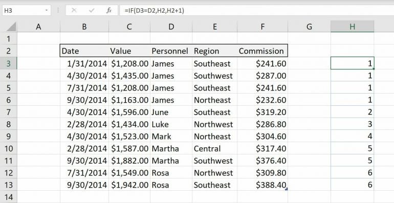
Now, let’s get started. Using the sheet in Figure A, enter into G3 the following function
=IF(D3=D2,H2,H2+1)
and copy it to the remaining cells. If you’re using a Table object, Excel will automatically extend the Table to include this new column if you add this function to column G; you don’t want that to happen. As you can see in Figure B, the helper value increases by 1 every time the value in the Personnel column changes.
Figure B
It’s worth mentioning that other expressions will work, but I chose this one because the consecutive numbers are a visual clue to what they represent. With the helper column in place, it’s time to add the conditional format rule.
An Excel conditional format rule
Finally, it’s time to create the conditional format rule that fills alternating groups in the Excel Table:
- Select the data, B3:F13. (Don’t include the column of consecutive values in column H.)
- On the Home tab, click the Conditional Formatting dropdown (Styles group) and choose New Rule.
- In the resulting dialog, click the Use a Formula to Determine Which Cells to Format option.
- Enter the function ISODD($H3) into the formula control in the lower pane.
- Click Format and then click the Fill tab.
- Choose a color—I chose light blue. When choosing, make sure it doesn’t clash with the sheet’s background, which will serve as the alternating color.
- Click OK to see the function and format shown in Figure C.
- Click OK to return to the Excel sheet.
Figure C
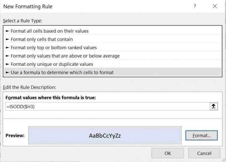
Figure D shows the applied format.
Figure D
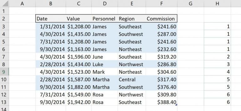
Keep in mind that you will need to re-sort when you modify the records by changing the Personnel value in an existing record or by adding a new record. When adding new records, you must extend the expression in the helper column.
SEE: Why Microsoft Lists is the new Excel (TechRepublic)
At this point, you could be done, because the white is an alternate color. However, you might want to apply a second color.
How to add another color in Excel
Right now, Excel is applying only one fill color. The even-numbered groups remain white—or whatever color the sheet background is. To add another color instead to fill the unformatted groups, repeat the above steps. In step 4, enter ISEVEN($H3), in step 6 choose a second color. As you can see in Figure E, I chose a light green, and Figure F shows the results.
Figure E
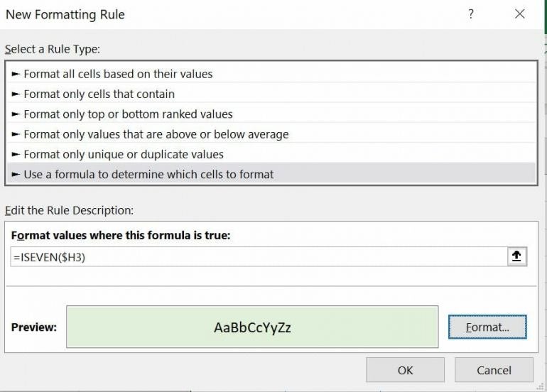
Figure F
To me, this technique seems a bit unfinished because the user must expand the helper column as they add new records. In addition, the conditional format rule doesn’t allow you to choose a different group. To do so, you must update the function in the helper column. However, if you want highlighted groups, this is an easy way to get them.