
The article How to concatenate values in a single Excel column to a single row shows you how to combine columnar data into a single Excel cell. It’s an odd technique, but data uses often require a different structure than we’re used to using in Microsoft Excel.
Fortunately, it isn’t difficult to transpose column values into a single cell as long as you don’t want to group the results. In that situation, you can use Microsoft Excel Power Query. In this tutorial, I’ll show you how to use Microsoft Excel Power Query to combine values into a single cell, within groups.
SEE: Windows, Linux, and Mac commands everyone needs to know (free PDF) (TechRepublic)
I’m using Microsoft 365 on a Windows 10 64-bit system. Power Query is available as part of the interface through Excel 2016. Excel for the web doesn’t support Power Query, but you can run existing queries in an Excel workbook.
How to load the Excel data into Power Query
When using Microsoft Excel’s Power Query, the first step is to load the Excel data into Power Query. If you’re not working with a Table object, Power Query will prompt you to convert the data range to a Table because Power Query works only with Excel Table objects.
The example data is in a Table named TableSales. You don’t have to name the Table, but a descriptive name does make a Table easier to work with, especially when there’s more than one.
Let’s start by adding the data in TableSales to Power Query:
- Click anywhere inside the Table.
- Click the Data tab.
- In the Get & Transform data group, click From Table/Range.
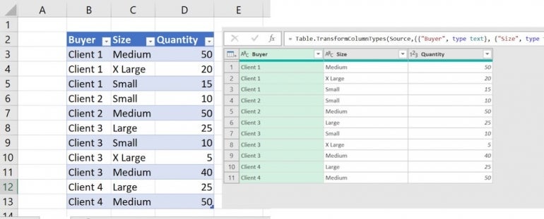
That’s all there is to it. Figure A shows the data in Power Query.
Figure A
How to add a new column in Power Query
Our goal is to combine the t-shirt sales by client into a single cell for each client. Doing so entails grouping by the clients. For example, for Client 1, we want one row with a column that combines the sales as follows: Medium: 50, X Large: 20, Small 15. To accomplish this, we need to add a new column for the combined values as follows:
- Hold down the Shift key as you click the Size and Quantity columns to select both.
- Click Transform in the Table group and then click Columns Merge in the Text Column group.
- In the resulting dialog, choose Custom from the Separator dropdown. We’ll use custom because we want to use a colon and space as the separator and that option doesn’t exist in the dropdown.
- In the next control, enter the character you want to separate the size and quantity. I entered a colon and a space character. You can’t see the space, it’s there.
- Enter a meaningful name, SizeQuantity, for the new column (Figure B).
- Click OK to see the results shown in Figure C.
Figure B
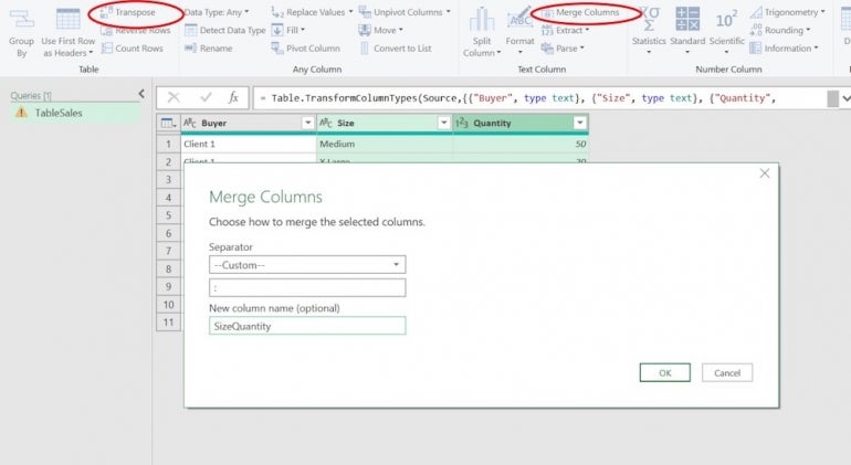
Figure C
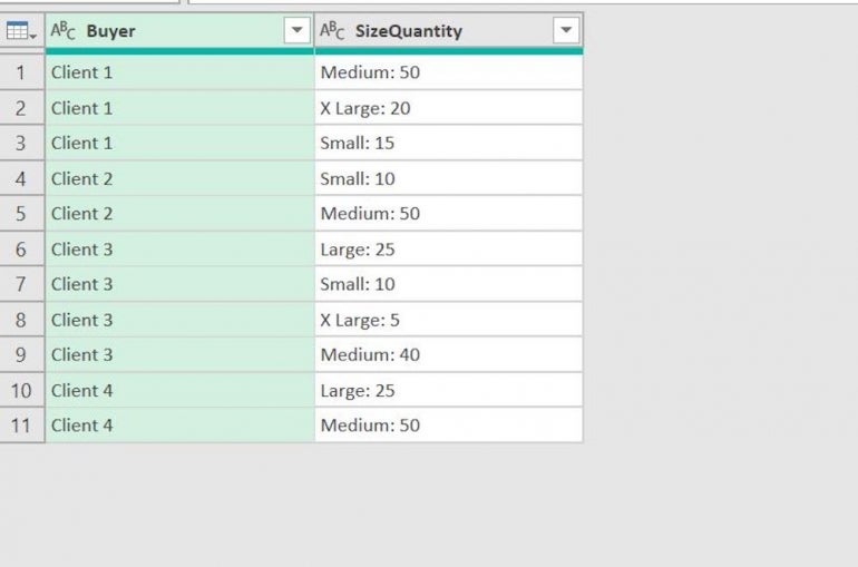
As you can see, this task combined the size and column value for each record. Now, we want to combine these values into one row for each client. That entails grouping.
How to group in Power Query
Right now, we have the size and quantity values combined in a single cell for each record. The next step is to group the data in Power Query by the Buyer (client) values, as follows:
- Select the header for the Buyer column to select it.
- Click Group By in the Table group. In the resulting dialog, the Basic option is the default because the selection contains only one column.
- Identify the column by entering SizeQuantity1 in the New Column Name field.
- From the Operation dropdown, choose Sum. This will generate an error, but we’ll modify the formula directly to correct it.
- Choose SizeQuantity from the Column dropdown (Figure D).
- Click OK.
Figure D
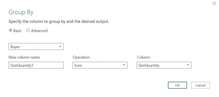
Figure E
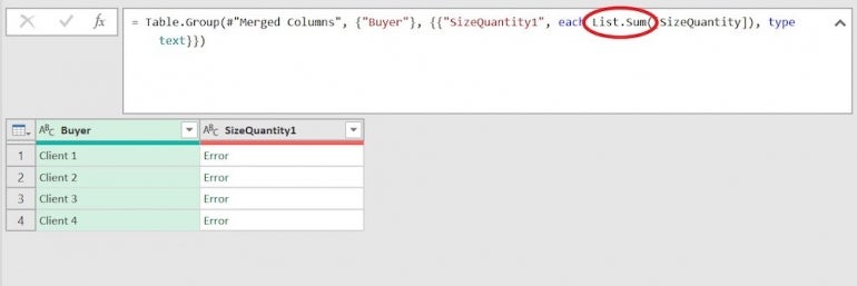
As you can see in Figure E, the task grouped the clients, but the Sum operator returns an error. To correct this error, we must modify the formula. Specifically, we must replace List.Sum with Text.Combine, which requires a separator argument.
To add this character, position the cursor after the closing bracket following SizeQuantity1 and before the closing parenthesis and enter the following as shown in Figure F: , "; ".
Figure F

After restructuring the data, you can return it to an Excel sheet.
How to load the Power Query data into Microsoft Excel
Power Query restructured the data as required. You have one record for each client and a cell that contains all the size and quantity data for the corresponding client. At this point, you can load it back into Microsoft Excel as follows:
- In Power Query, click the Home tab.
- In the Close group, click Close & Load.
Figure G

As you can see in Figure G, Power Query saves the table in a new Excel sheet. At this point, you can use the data or pass it along.
Using Power Query to restructure Microsoft Excel data requires no expressions or functions. You add a column for the combined values and then group if you want to combine those values further into a single record.
