An Excel drop-down list can make it easier for the average Microsoft Excel user to enter data. Using a drop-down limits the entry choices for a selected cell, speeding data entry and reducing data entry error. In this article, I’ll show you a quick and easy way to create a drop-down list using Excel’s Data Validation feature.
SEE: Windows, Linux, and Mac commands everyone needs to know (free PDF) (TechRepublic)
I’m using Microsoft 365 desktop on a Windows 10 64-bit system, but you can use an earlier version. For your convenience, you can download the demonstration .xlsx and .xls files.
However, the Table object isn’t available in the older menu versions (.xls) so some of this article won’t apply if you’re still using an .xls version. You can still use a data range for the list, but the populated drop-down won’t update when you update the list items. Microsoft Excel for the web supports data validation and you can even add a data validation drop-down list in the web version. You can’t expand an Excel Table by tabbing through the cell to insert a new row, but you can still add a row.
What is a drop-down list in Excel?
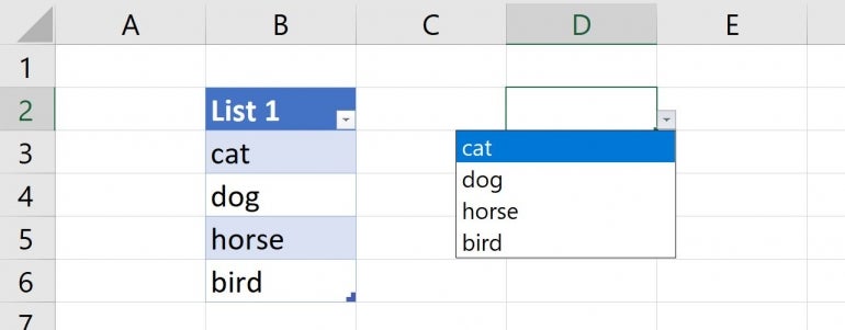
Figure A shows a simple drop-down list in an Excel sheet. To use the drop-down, click the data entry cell (D2 in this case) and then click the drop-down arrow to display the list of values in B3:B6. If a user tries to enter something that isn’t an item within that list of values, Excel rejects the entry, protecting the validity of your data.
Figure A

To create a data validation drop-down list in Excel, you need two things: A list of values and a blank cell to use as the data entry cell. The list is in B3:B6 and the data entry cell is D2.
How to add a data validation drop-down in Excel
Now that you know how users and your data will benefit from a drop-down list, let’s add one to D2. First, add the short list (Figure A) to B3:B6 and format it as an Excel Table object. Simply click any cell in the list and press Ctrl + T. In the resulting dialog, make sure the My Table Has Headers option is selected, and click OK. Technically, the list items don’t need to be formatted as a Table, but a Table makes the drop-down dynamic.
To add the drop-down list in our example to an Excel cell, do the following:
- Select D2 to follow the example, but you can put the drop-down anywhere.
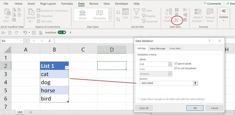
- Click the Data tab and then click Data Validation in the Data Tools group. Click the Settings tab, if necessary.
- In the resulting Data Validation dialog, click List from the Allow options drop-down.
- Click the Source control and highlight B3:B6 — the list items.
- Click OK.
Figure B

Click the drop-down to see the list shown earlier (Figure A).
You can add a drop-down to multiple Excel cells. Select the range of data input cells (Step 1) instead of a single Excel cell. Doing so will populate multiple drop-downs with the same list items. It even works for noncontiguous Excel cells. Hold down the Shift key while you click the appropriate Excel cells. The average user won’t benefit from this added functionality, but it’s good to know that it’s possible.
SEE: Why Microsoft Lists is the new Excel (TechRepublic)
Earlier, you formatted the list items as a Table object. Now, let’s discover why by entering a new list item into the Table:
- Select B6 and press Tab to add a new cell to the Table.
- Enter “goat” and press Enter.
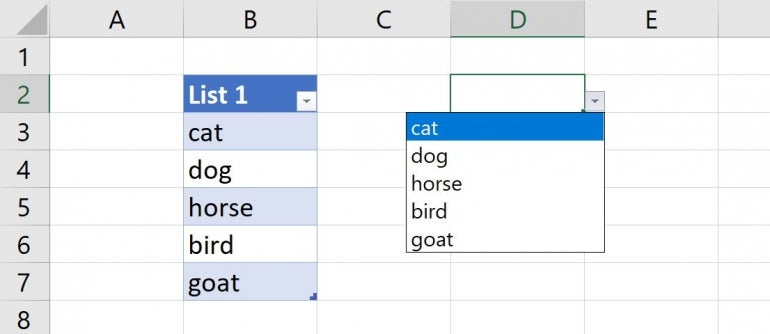
Excel added “goat” to the drop-down list (Figure C). You didn’t have to do a thing, other than enter the new list item. That’s the power of Excel’s Table object. I recommend that you use them whenever possible. To remove an item from the drop-down, remove it from the Table.
Figure C

How to use a drop-down in an Excel Table
We can expand on the Table topic, because if you add a data validation drop-down to the first cell in a Table, Excel will extend the drop-down to each new record. Let’s take a quick look at this bit of magic:
- Create a quick Table by selecting F2:G4. Then, press Ctrl + T, click the My Table has Headers option, and click OK.
- Select D4, the cell with the drop-down we created earlier, and press Ctrl + C.
- Select G3, the first cell in that column and press Ctrl + v to copy the drop-down to that cell.
The drop-down is available in the first cell in column G (Figure D).
Select an item from the drop-down and then press Tab to insert a new record into the Table. Tab to G4 and you’ll see that the Table copies the drop-down automatically (Figure E). If you’re using Excel for the Web, right-click the Table, choose Insert from the resulting submenu, and then select Table Rows Above. The web version will copy the drop-down as the desktop version does.
Figure D

Figure E

You could’ve created the data validation list using the interface, as you did earlier. However, I want you to know how easy it is to copy a drop-down.
By now, you’ve probably noticed that you can only see the drop-down arrow if you click on the Excel cell. This is a bit of a deterrent. I recommend that you choose a format, such as a fill color, so it’s easy to find. Users must choose an item; if they try to enter their own data, they’ll trigger an error. There are options for displaying a specific error message, but we won’t cover that in this article.
Using multiple links to Microsoft Excel workbooks
It’s possible to populate a drop-down by referencing list items in another sheet or even another workbook. The process takes a bit of work, so we didn’t cover this option in this article.
Both workbooks must be open. If you try this, keep in mind that multiple links where values in workbook1 depend on values in workbook2, which links to workbook3, and so on, are hard to manage. Users forget to close files, and sometimes they even move files. If you’re the only person working with linked Excel files, you might not run into trouble, but if other users are reviewing and modifying them, you’re asking for difficulty. If you truly need that much linking, you might consider a new design.
Stay tuned
In a future article, I’ll show you how to populate a drop-down in one workbook by referencing items in another workbook. Linking between workbooks isn’t difficult, but it isn’t intuitive.


