


Must-read big data coverage
- What Powers Your Databases? Take This DZone Survey Today!
- New AI Data ‘Universal Translator’ From Salesforce, Snowflake, Others
- Top Tech Conferences & Events to Add to Your Calendar in 2025
- Google Releases Data Commons MCP Server to Supercharge AI Agents
Color can be a powerful element in an Excel drop-down list, and it’s easier to add than you might think. Perhaps you want to use a color to denote a specific group or task, or maybe you just want to draw attention to the control. Whatever your reason for incorporating color, you can accomplish your goal by simply adding conditional formatting to the cell that contains the drop-down list.
SEE: The Complete Microsoft Office Master Class Bundle (TechRepublic Academy)
In this tutorial, I’ll show you how to add a validation control and then add conditional formatting to include visual cues for the drop-down. Throughout this article, we’ll use Excel’s built-in data validation drop-down control rather than a development, legacy combo or list control.
I’m using Microsoft 365 on a Windows 10 65-bit system, but you can use earlier versions of Excel or Excel’s online version as well. You can work with your own data or download the demonstration files I’m working with here.
Jump to:
- How to add color to an Excel drop-down list
- Creating an Excel drop-down list
- How to change the font color for an Excel drop-down list
- How to change the color of a cell in an Excel drop-down list
- Get more Excel tips
How to add color to an Excel drop-down list
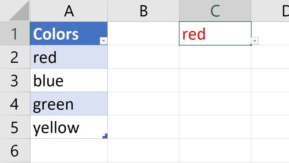
If you’ve used data validation controls, you know how easy they are to add and how helpful they can be. This type of control is truly one of Excel’s most helpful features, because the drop-down list can be almost anything. In this case, we’ll use a list of color names at the sheet level. To accomplish this, enter the list of color names shown in Figure A.
Figure A
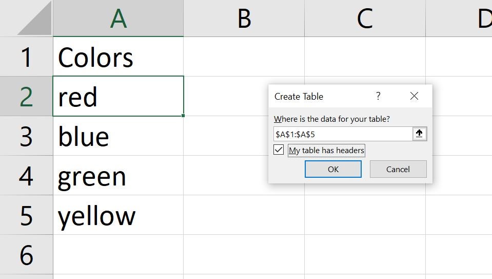
This next step isn’t necessary for this technique to work, but it will help you work more efficiently. Format the simple list as a table object by clicking anywhere inside the list and pressing Ctrl + T or by choosing the Format as Table option in the Home tab.
SEE: Checklist: Microsoft 365 app and services deployments on Macs (TechRepublic Premium)
Check the My Table Has Headers option, and click OK. Doing so will make the drop-down list dynamic. When you update the list at the table (sheet) level, Excel will automatically update the list in the drop-down.
Now, let’s add the drop-down list and populate it with the list of color names in A2:A5.
Creating an Excel drop-down list
To illustrate how easy these lists are to add and populate, let’s add one that displays the list of colors in A2:A5. When applying this technique to your own work, you’ll probably use meaningful group or task names. I’m using colors to help visualize what happens when you choose from the list of color names in the drop-down.
The next step is to add the drop-down list as follows:
- Select the cell where you want to display the drop-down. For our demonstration, I’ve chosen C1.
- Click the Data tab.
- In the Data Tools group, click the Data Validation option. If you clicked the drop-down, choose Data Validation.
- In the resulting dialog, choose List from the Allow drop-down options.
- In the Source control, enter $A$2:$A$5 (Figure B), or you can select the list. Then, click OK.
Figure B
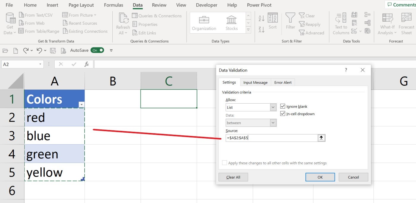
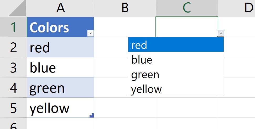
Figure C shows the new list. If you choose an item, Excel will display it in the control, but you don’t need to select a color name at this time.
Figure C
As mentioned, the data validation control feature is versatile. When you have a bit of time, you might want to return to this feature and check out the many ways you can specify the values that populate the list.
With this new list in place, you’re ready to add conditional formatting.
How to change font color for an Excel drop-down list
We’re going to combine the data validation control with the conditional formatting feature in order to apply a font color to the selected list value. Specifically, the rule will apply the font color represented by the color name: red font for the name red, blue for the name blue and so on. Fortunately, there’s a predefined rule that will help us complete this task.
SEE: 108 Excel tips every user should master (TechRepublic)
The thing to remember is that the data validation control links to cell C1, and the conditional formatting rule we’re going to add is set for cell C1. We’re not really changing the color of anything in the drop-down list itself. We’re changing the color of the selected value, which Excel displays in C1.
Now, to specify a conditional rule that changes the font color of a list item, do the following:
- With C1 selected, click the Home tab; C1 is the same cell where we put the data validation control.
- In the Styles group, click Conditional Formatting.
- Choose New Rule from the submenu.
- In the top pane, select the Format Only Cells That Contain option.
- In the lower section, change the first drop-down setting (Cell Value) to Specific Text, which updates the second control to Containing. If that doesn’t happen for you, select Containing from the second drop-down.
- In the third control, enter =A2, the cell that contains the text value red.
- Click the Format button.
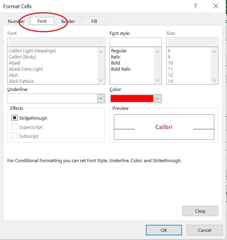
- In the resulting dialog, click the Font tab, choose red (Figure D) and click OK. Then, click OK again to return to the sheet.
Figure D
If you select red, the font color is red, as shown in Figure E. When selecting the other three list items, the font is black because those list items don’t have a conditional formatting rule yet.
Figure E
To finish the list, create a rule for each item in Table A. Simply repeat the instructions above, but enter the appropriate cell reference in step 6, and then, choose that color in step 7. If a rule doesn’t work for you, make sure you include the equals symbol (=) in the cell reference.
Table A
| Color | Cell value | Second control | Cell |
|---|---|---|---|
| Blue | Specific Text | Contains | Green |
| Green | Specific Text | Contains | Yellow |
| Yellow | Specific Text | Contains | 0 |
Changing the font color is one way to represent the selected item in the drop-down. You could just as easily use the Fill property instead.
How to change the color of a cell in an Excel drop-down list
In the last section, you used conditional rules to change the font color. In this section, I’ll show you how to apply the Fill property instead. Doing so will apply the specific color to the cell’s background rather than the font.
To do so, you’ll need to recreate the list and data validation control on a new sheet or delete the rules and validations we’ve used in previous steps to start afresh. Although it isn’t impossible to mix the rules on the same sheet, doing so requires some rather complex rules.
SEE: 30 Excel tips you need to know (TechRepublic Premium)
The change is simple to make. Repeat steps 1 through 7 above. Then in step 8, you’ll click the Fill tab and choose red, as shown in Figure F.
Figure F
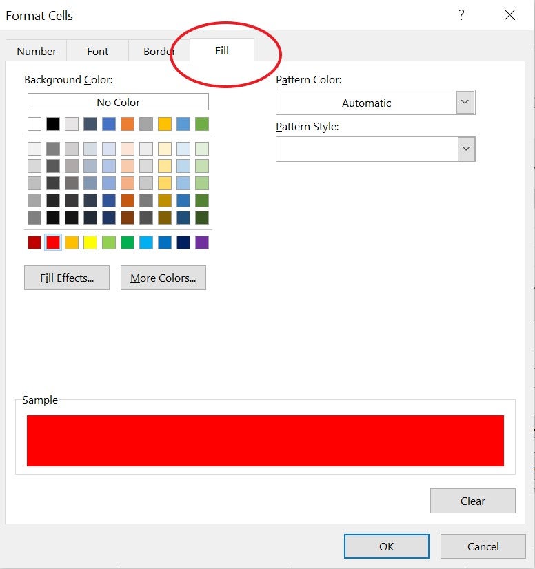
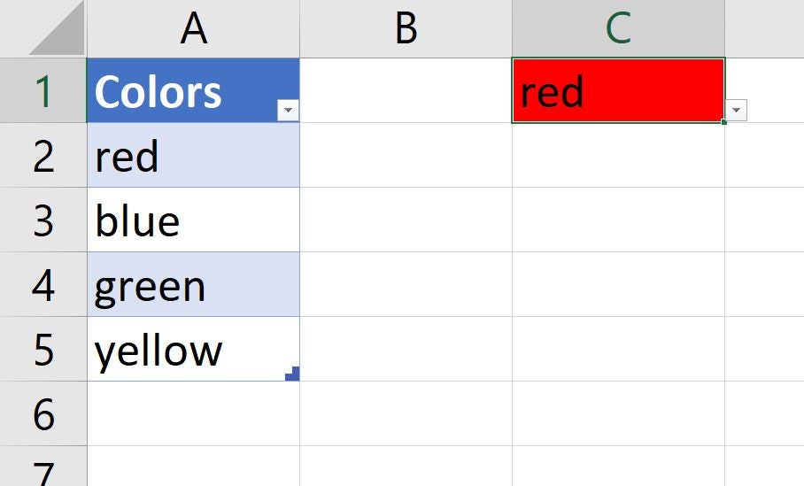
When you choose red from the list, the rule will apply the color red to the Fill property (Figure G). In this case, the font color remains black, and the background color will update to your selected color.
Figure G
Adding color is a helpful visual tool, whether you’re trying to identify the drop-down cell or a selected item from the list. The demonstration file contains both drop-downs, complete with all rules.
Get more Excel tips
Excel’s data validation control feature is easy to use and helpful. If you’d like to learn other ways to put this feature to work for you, consider reading the following articles:
- How to create a drop-down list in Excel (TechRepublic)
- How to use UNIQUE() to populate a drop-down in Microsoft Excel (TechRepublic)
- How to create an Excel drop-down list from another tab (TechRepublic)
TechRepublic has an extensive library of other Excel and Microsoft tutorials as well. To learn more about how to use Microsoft Office products and their functions to your advantage, take a look at our Microsoft tutorial library here. We also offer several Microsoft education programs and certifications through TechRepublic Academy.
Read next: The best project management software and tools (TechRepublic)