


Many solutions require more than a simple function or filter. For instance, if your company applies stipends for travel, you probably add the same amount for every employee for travel days. Now, let’s suppose that your company pays a different stipend for each job site location and that an employee could earn more than one stipend in a single day? The solution isn’t as difficult as it sounds, but it’s more complicated than using an IF() statement to add a fixed amount on travel days.
In this article, we’ll combine a VLOOKUP() function, a data validation list, and a PivotTable to create a simple application that tracks stipend awards for employees when working at off-site job locations. The structure is flexible enough to accommodate employees who work at multiple off-site locations in a single day. The VLOOKUP() function will return the correct stipend for each location record. A data validation control will restrict input to specific sites, avoiding typos and invalid sites. Finally, a PivotTable will return stipend totals earned for each employee by employee and date.
More about Software
- Software Installation Policy
- Five Methods to Insert a Checkmark Into Microsoft Office Products
- How to Hide and Handle Zero Values in an Excel Chart
- How to Use Section Breaks to Control Formatting in Word
I’m using Office 365’s Excel (desktop), but you can use earlier versions. You can work with your own data or download the demonstration .xlsx and .xls files. Unlike many solutions, you can create and use this solution in the browser edition. You don’t need to know anything about the VLOOKUP() function or how to create a validation list or PivotTable but being familiar with these features will be helpful.
SEE: Choosing your Windows 7 exit strategy: Four options (Tech Pro Research)
The problems
The simple sheet shown in Figure A contains two Table objects. The one on the left tracks the hours each employee works at specific work sites. The Table to the right lists each site and its daily stipend. You could memorize the amounts and list them with the hourly record, but that invites trouble: You might enter the wrong amount, and anytime you enter values manually you risk typos. By having a stable list, you ensure the validity of your data. But, how do match them? The simplest answer is to use a VLOOKUP() function.
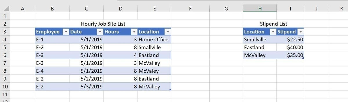
There are a few things worth noting before we continue:
- Each employee might visit one or more job sites in a single day. That means we’ll have to add those amounts into a single daily stipend total.
- Each employee might spend a few hours or the entire day at the home office, which has no stipend.
- Data entry is very important. The location value in the hourly list must match a location value in the stipend list to avoid errors.
Throughout the article, I’ll refer to the list on the left as the hourly list and list on the right as the stipend list. We’re working with Table objects so we can easily modify the Stipend List without updating its references. To convert a regular data range into a Table object, do the following:
- Click anywhere inside the data range.
- Click the Insert tab and then click Table in the Tables group.
- Indicate whether the data has headers (the demonstration data does).
- Click OK.
If you’re working with your own data, you don’t have to use Table objects, but the remainder of this article assumes you are.
The VLOOKUP() function
The quickest way to add a stipend amount for each job site to the hourly list is to add a VLOOKUP() function using the following syntax:
VLOOKUP(lookup_value, table, column_index, range)
where lookup_value is the cell or range that contains the value in the hourly list that you’re looking up–Location (column E) in this case; table identifies the lookup table–H4:I6 (the stipend list Table minus the headers); column_index represents the column that contains the values you want to return in relation to the lookup value–Stipend, and range is a TRUE/FALSE value that forces (or not) an exact match.
Now, let’s enter the following VLOOKUP() function into cell F4:
=VLOOKUP([Location],Table2,2,FALSE)
If you’re not working with Table objects, enter this function instead:
=VLOOKUP($E$4:$E$10,$H$4:$I$6,2,FALSE)
Note that the two ranges (for a regular data range) must be absolute references.
Figure B shows the results after formatting the new column as Currency and adding header text. The Table will automatically adjust to include the new column.
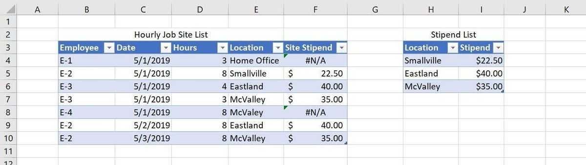
We have two apparent problems: The home office and McValey (row 8) both return the same error message. The error in row 4 is easy to fix; the error in row 8 will require a bit more work.
Problem 1
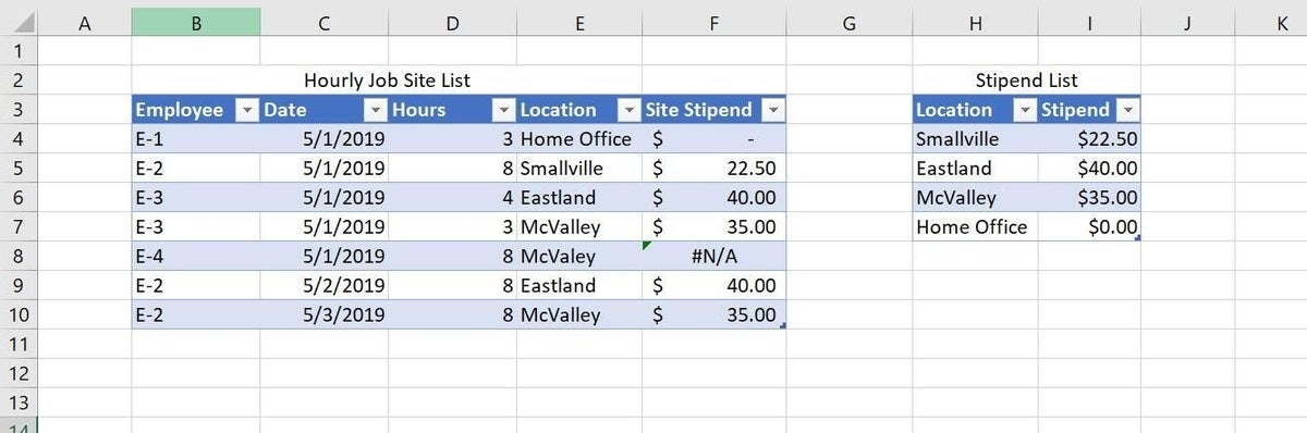
Excel returns an error in row 4 because there’s no matching location value in the stipend list. To fix this error, simply add a new record to the stipend list, as shown in Figure C. As you can see, this simple fix takes care of the error in row 4. This is why I chose to use Table objects–the VLOOKUP() function automatically updates to include the new row–you don’t have to modify the function.
Problem 2
The error in row 4 was easy to troubleshoot and fix. Can you determine why the VLOOKUP() function for row 8 returns an error? There’s a record for the McValley job site in the stipend list, so the next place to look is the location value in the hourly list. Does it match, exactly, the value in the stipend list? Oh! That’s right, it’s missing an l–the location is misspelled.
The easiest solution is to fix the typo, but that won’t eliminate new typos in the future. Instead, let’s add a data validate list to the hourly table. Doing so will limit users to items in the list and avoid future errors. Specifically, the list will include the location values from the stipend list, and you’ll enter the location using the list instead of manually typing each location.
Add the list as follows:
- Select E4:E10 (If you add the validation list to E3, it won’t add a control to existing or new records.)
- Click the data tab and then click Data Validation in the Data Tools group.
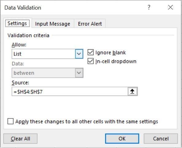
- In the resulting dialog, choose List from the Allow dropdown.
- Indicate the location values in the stipend group in the Source control (Figure D).
- Click OK.
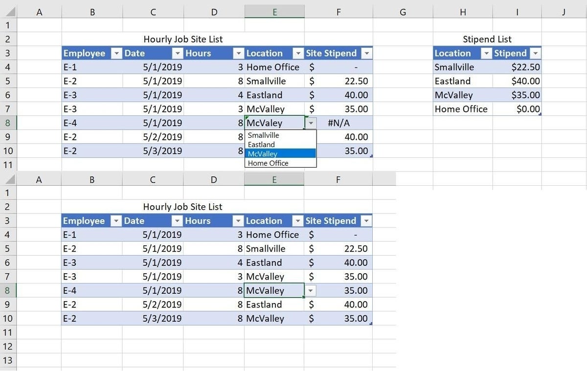
Now, select E8 and using the validation control’s drop-down list, enter McValley, as shown in Figure E. As you can see, once you correct the spelling of the location value, the VLOOKUP() function works as expected. In addition, the control is dynamic–more Table magic. Updating the stipend list will also update the validation control’s list. You can’t do that with an ordinary data range.
To learn more about VLOOKUP() errors, read Troubleshoot VLOOKUP() formula gotchas.
The daily totals
After fixing the two problems inherent to the original structure, we now have stipend totals for each site record. However, the current hourly list structure doesn’t return a daily total for each employee. Remember, each employee can work at more than one location in the same day. For example, E-3 worked at two sites on May 1 and both sites have applicable stipend rates. E-3 should receive a total of $75 in stipend rates for May 1–not $40 or $35 (the individual location rates).
There are a number of ways to accomplish this, but perhaps the easiest is to use a PivotTable. To do so, click anywhere inside the hourly list and click the Insert tab. Then, do the following:
- Click PivotTable in the Tables group. In the resulting dialog, click OK.
- Click inside the PivotTable frame, which will display the list pane.
- In the fields pane, check the Employee and Site Stipend fields (Figure F).
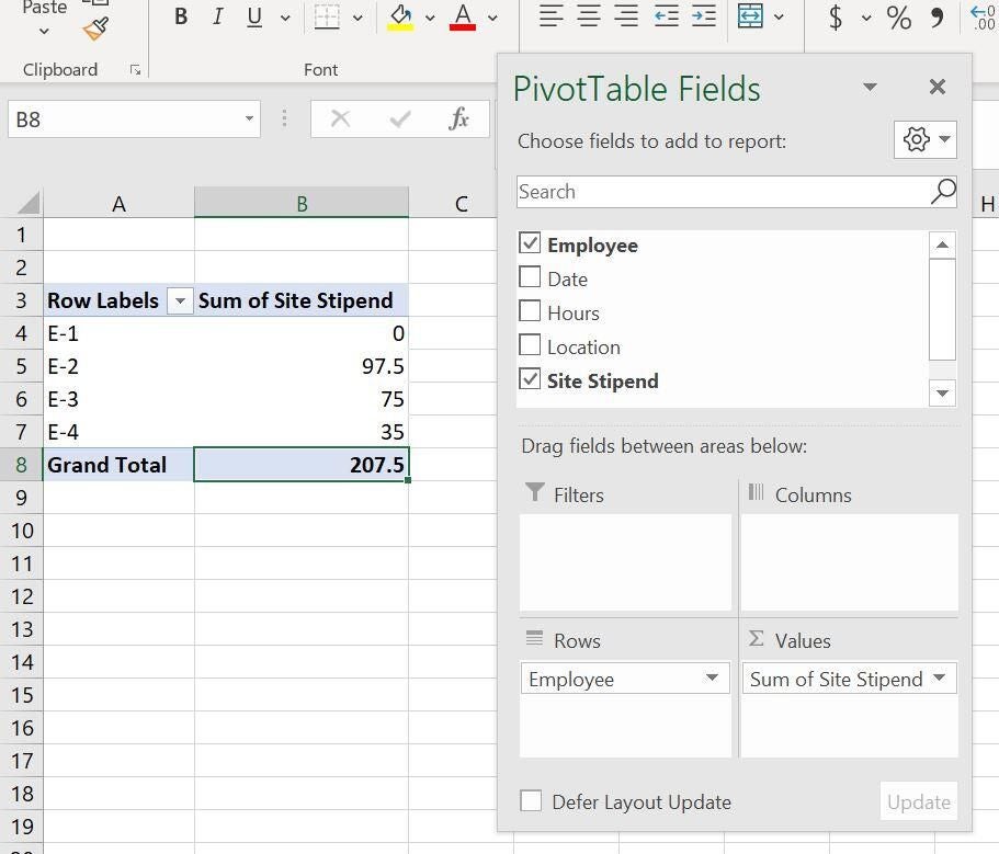
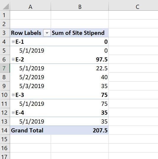
As is, the PivotTable displays grand totals for each employee. As you can see in Figure F, E-3’s total is $75–the addition of two sites on the same day. If you need a daily subtotal, add the Date field to the PivotTable, as shown in Figure G.
To learn more about PivotTable objects, read Get the most out of your Excel PivotTables with these handy tips.
Combo solution
As is often the case, an efficient solution required a combination of efforts. In this case, we used the VLOOKUP() function to add an important detail to a tracking list. Specially, we added a stipend amount for each location worked. Then, we used a PivotTable to add those stipend rates in two different ways. In a future article, we’ll continue this solution scenario by using Power Query.
Send me your question about Office
I answer readers’ questions when I can, but there’s no guarantee. Don’t send files unless requested; initial requests for help that arrive with attached files will be deleted unread. You can send screenshots of your data to help clarify your question. When contacting me, be as specific as possible. For example, “Please troubleshoot my workbook and fix what’s wrong” probably won’t get a response, but “Can you tell me why this formula isn’t returning the expected results?” might. Please mention the app and version that you’re using. I’m not reimbursed by TechRepublic for my time or expertise when helping readers, nor do I ask for a fee from readers I help. You can contact me at susansalesharkins@gmail.com.
See also
- How to use conditional fields in a Word mail merge (TechRepublic)
- Office Q&A: Collapsible heading and delay send settings aren’t a cure all, but it’s close (TechRepublic)
- How to document Word AutoText and AutoCorrect entries (TechRepublic)
- How to document Word keyboard commands (TechRepublic)
- How to turn ordinary sparklines into meaningful information with a few simple formats (TechRepublic)
- 10 free alternatives to Microsoft Word and Excel (TechRepublic download)
- Microsoft Office 365 for business: Everything you need to know (ZDNet)
- The 10 most important iPhone apps of all time (Download.com)
- It takes work to keep your data private online. These apps can help (CNET)
- Programming languages and developer career resources coverage (TechRepublic on Flipboard)