Image: iStock/muchomor
One of the most common requests I receive from users is how to identify duplicate and unique values in Microsoft Excel. The easiest way I know is to apply a conditional format. In a nutshell, a conditional format changes the appearance of cells or values based on true/false conditions that you specify. For example, a teacher might set a conditional format to display GPAs below 75 in red. Doing so would visually alert her to students who aren’t doing well in her class. In this article, I’ll show you two ways to highlight unique values using conditional formatting. First, we’ll review the easy way: Using a built-in rule that highlights the individual value. Then, we’ll use a conditional format formulaic rule that highlights the entire record.
SEE: 60 Excel tips every user should master
I’m using Microsoft 365 on a Windows 10 64-bit system, but you can use an earlier version. You can work with your own data or download the demonstration .xlsx file. The browser supports conditional formatting; however, you can’t use the browser to implement a formula rule.
How to highlight values
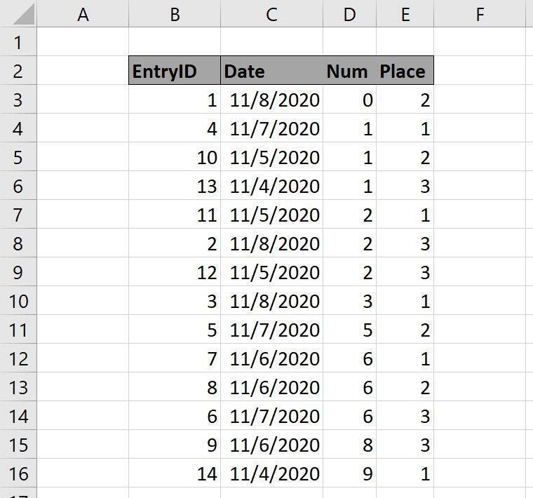
Excel has a built-in conditional rule that highlights unique values. You don’t have to come up with a special formula—you just run though a few clicks. The hardest part is finding it! Using the sheet in Figure A, let’s use this rule to identify the unique values in the Num column:
- Select the values you want to format; in this case that’s D3:D16.
- Click the Home tab. Then, click the Conditional Formatting dropdown in the Styles group.
- From the dropdown, choose Highlight Cells Rules, and then choose Duplicate Values from the resulting submenu (Figure A). Earlier, I said this rule is hard to find—you might not think to look for a unique rule under a duplicate rule.
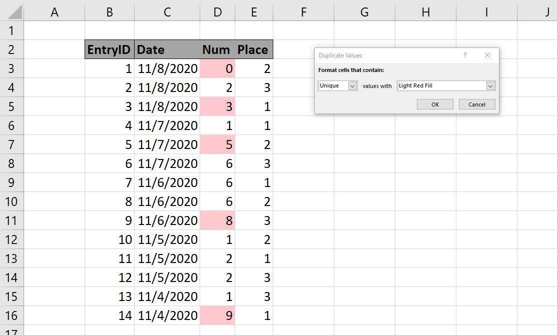
- The dropdown to the left defaults to Duplicate, but you can choose Unique.
- Then, choose a preset format from the dropdown to the right (Figure B).
- When you click OK, Excel highlights the unique values in the range you selected in step 1.
Figure A
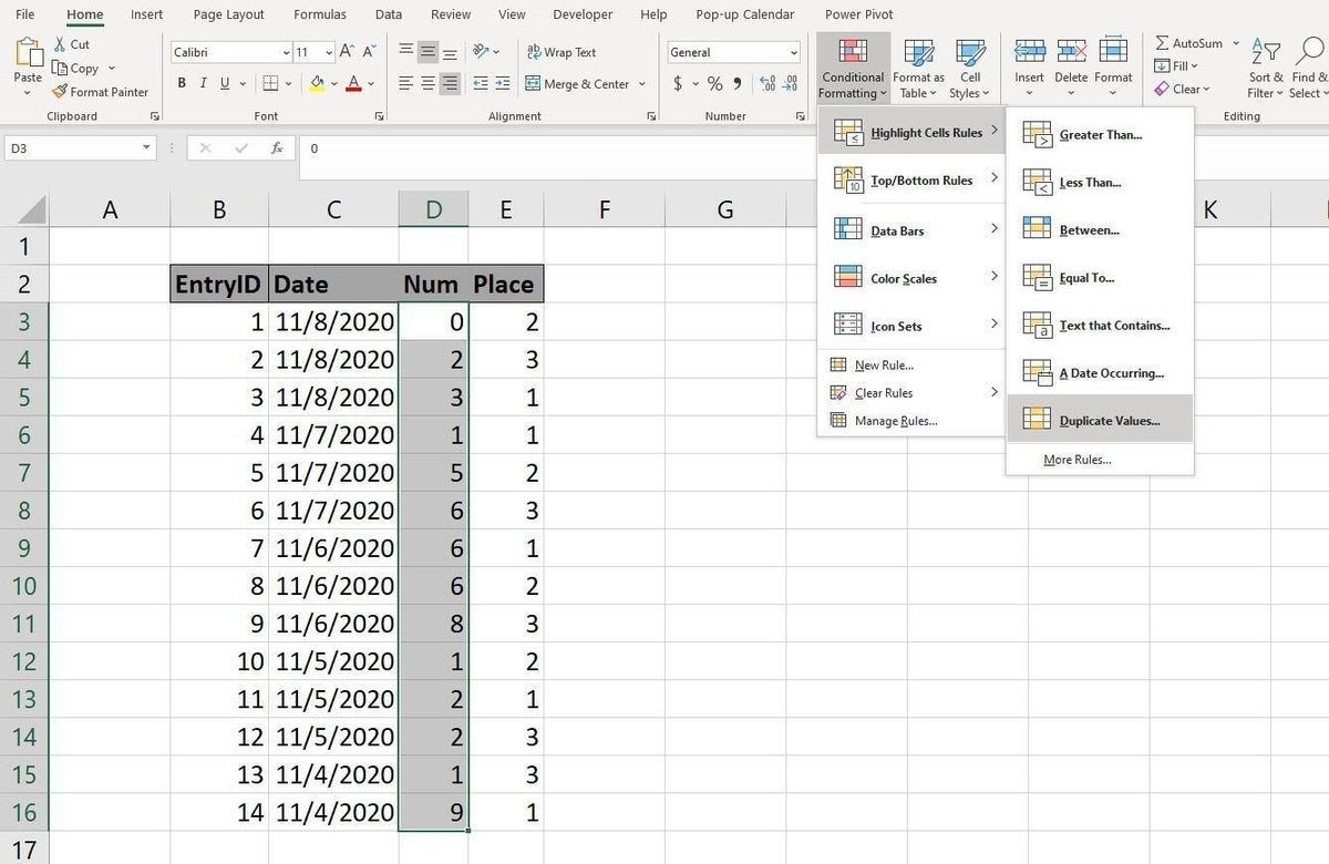
Figure B
It’s super easy to implement, but as you can see, this method highlights only the values, which can be visually challenging. Highlighting the entire record helps the user find corresponding values quicker.
SEE: How to easily include dynamic dates in a Word doc using Excel (TechRepublic)
How to highlight rows
There’s no built-in rule that will highlight the entire record. For that, you’ll need a formula that returns true when the value is unique and false when the value is a duplicate. To accomplish this, we’ll use the COUNTIF() function in the form:
COUNTIF(range,criteria)
where range identifies the entire data set (record) and criteria specifies the condition, which can be a cell reference, a value, or even an expression. The COUNTIF() function counts the number of cells in range that satisfy criteria. Now, we don’t want a count, but we know that a unique value will return the value 1. Let’s try that now:
- Enter the following function into cell H3 and copy it to the remaining cells:
=COUNTIF($D$3:$D$16, $D3) - As you can see in Figure C, this function returns 1, when the corresponding value in column D is unique. We can quickly turn this into a true/false result using the function
=COUNTIF($D$3:$D$16, $D3)=1 - Figure D shows the results: The function returns true when the corresponding value is 1 and false when it’s any other value. By the way, you can use the same function to find duplicates by simply changing the equality operator from = to <>.
Figure C
Figure D
The next step is to enter the true/false expression as a conditional rule:
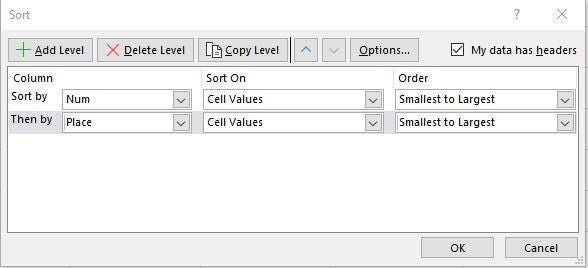
- Select the data range, B3:E16–you want to highlight the entire row. If you use a Table, Excel will update range as you add and delete records. The demonstration file contains a Table example.
- Click Conditional Formatting in the Styles group and choose New Rule.
- In the top pane of the resulting dialog, click the last option, Use a Formula to determine which cells to format.
- In the bottom pane, enter the formula
=COUNTIF($D$3:$D$16, $D3)=1 - Click Format, click the Fill tab, choose red from the palette, and then click OK. Figure E shows the rule and a preview of the format.
- Click OK.
Figure E
As you can see in Figure F, this rule highlights the entire row–the row is the same as before but it’s easier to discern all of the data that goes with the unique value. It’s not difficult to make a unique value (or duplicate for that matter) stand out, whether you want to see only the value or the entire corresponding record.
Figure F