


Last month’s article How to create an effective, user-friendly slicer in Excel offered an introduction to Excel’s slicer feature. This graphic tool lets users, with no specialized skill, filter data in a meaningful way. This month, we’ll continue our discussion of slicers with a more advanced topic: using a single slicer to update two or more PivotTables. Doing so is helpful when you want to focus on data in the same data source in different ways.
More about Software
- Software Installation Policy
- Five Methods to Insert a Checkmark Into Microsoft Office Products
- How to Hide and Handle Zero Values in an Excel Chart
- How to Use Section Breaks to Control Formatting in Word
I’m using Excel 2016 on a Windows 64-bit system, but the feature is available in Excel 2010 and 2013. In Excel 2010, slicers work only with PivotTables. Beginning with Excel 2013, you can add a slicer to a Table. They even work in a browser using Excel Web App. For your convenience, you can download the .xlsx demonstration file. (This file also contains the example data and slicer from last month’s article.)
SEE: Microsoft releases 64-bit Office for Mac: The secret to getting it
A quick preview
We’ll be working with the data shown in Figure A to create two PivotTables and then link the same slicer to both. The first PivotTable will sum the Value field by region; the second will sum the Commission field by personnel. The second PivotTable won’t even display the region, but the slicer will still filter it by region.
Figure A
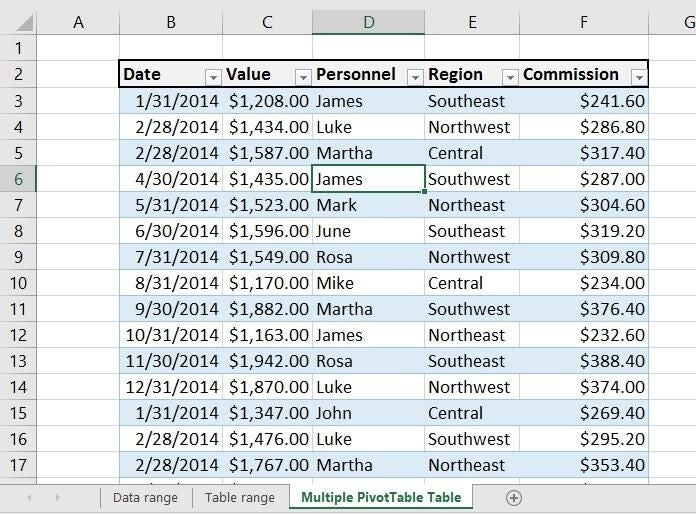
We’ll use this data to create our two PivotTables.
Although the entire process is simple to implement, there are several steps. It might be helpful to know what to expect:
- We’ll create the first PivotTable.
- We’ll copy the first PivotTable to create a second PivotTable.
- We’ll name both PivotTables.
- We’ll base a slicer on one PivotTable.
- We’ll link the slicer to the second PivotTable.
- We’ll format the PivotTables and sheet to resemble a dashboard environment (sort of).
Generate a PivotTable
We’ll begin by generating the first PivotTable. If you’re using Excel 2016, Excel does almost everything for you. To generate the first one, do the following:
- Click anywhere inside the Table (the demonstration file’s sheet name is Multiple PivotTable Table).
- Click the Insert tab and then choose Recommended PivotTables in the Tables group.
- Select the first option (Figure B), Sum of Value by Region, and click OK. Excel creates the selected PivotTable (Figure C) on a new sheet–I named the new sheet Multiple PivotTables, but doing so isn’t necessary.
Figure B
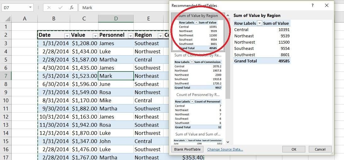
Select the recommended PivotTable.
Figure C
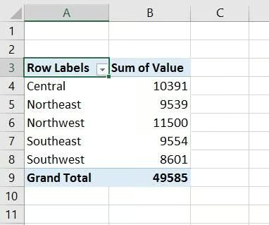
Excel adds the PivotTable to a new sheet.
I chose this route because it’s so simple. You don’t need to know anything about creating a PivotTable! If you need more help creating a PivotTable from scratch, see Make summarizing and reporting easy with Excel PivotTables.
You won’t create the second PivotTable using the recommended feature, or even from scratch. In fact, if you do, you won’t be able to connect the same slicer to both. You must copy the first PivotTable to create the second one and then change the second PivotTable’s settings.
To create the second PivotTable, do the following:
- Select the first PivotTable by clicking anywhere inside it and then clicking Select in the Actions group (on the contextual Analyze tab).
- Choose Entire PivotTable from the dropdown list.
- Press [Ctrl]+C.
- Click D3 and press [Ctrl]+V to paste a copy of the first PivotTable into the same sheet.
- In the PivotTable Fields pane (to the right), unselect Value in the top pane.
- Drag Commission to the Values control (Figure D).
- Uncheck Region in the top pane to remove it from the Rows control and then drag Personnel from the top pane to the Rows control.
Figure D
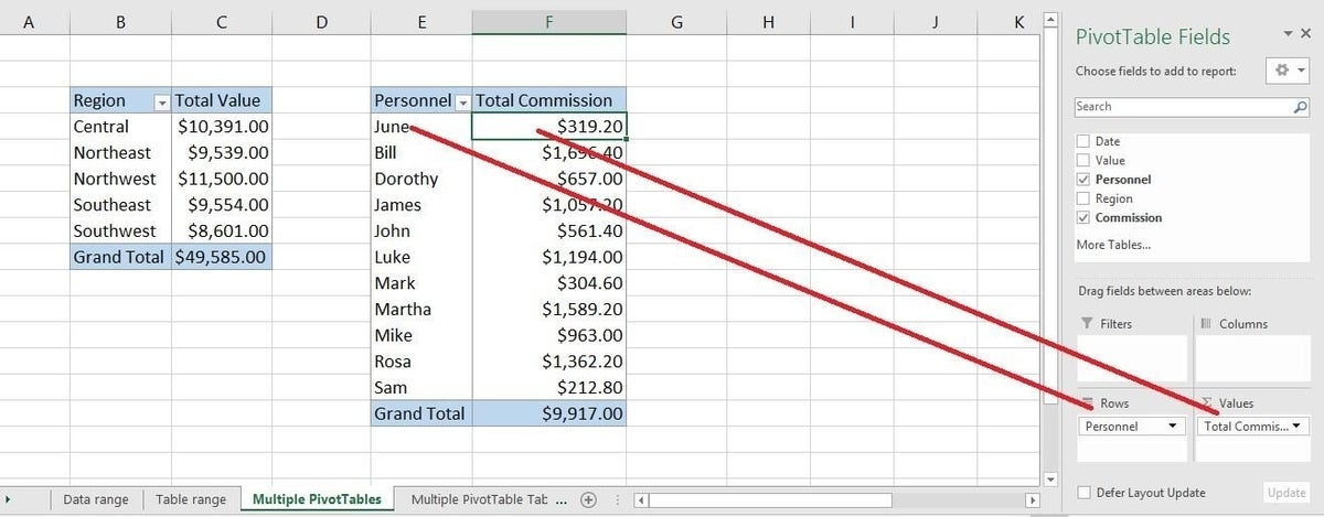
Copy the first PivotTable to create the second.
We now have two PivotTables based on the same data. I also changed the default header text labels to be more meaningful. This step isn’t necessary, but you should know how easy it is to change the default headings. The first sums the Value column by region; the second sums the Commission values for each person listed in the Personnel column.
It’s important to repeat at this point that this technique works only if you copy the first PivotTable. If you try to create the second PivotTable from scratch, you won’t be able to connect the same slicer to both PivotTables.
Name the PivotTables
Now that you have both PivotTables, you can name them. You don’t have to take this step, but doing so makes them easier to work with, especially if you have lots of PivotTables. To name them, do the following:
- Click anywhere inside the Sum of Value PivotTable.
- Click the contextual Analyze tab. On the far left you’ll see a default name for the PivotTable in the PivotTable group.
- Click inside that control and overwrite the default name. I named the first one, ptValue (Figure E). I recommend that you use meaningful names.
- Repeat steps 1 through 3 to name the second table ptCommission.
Figure E
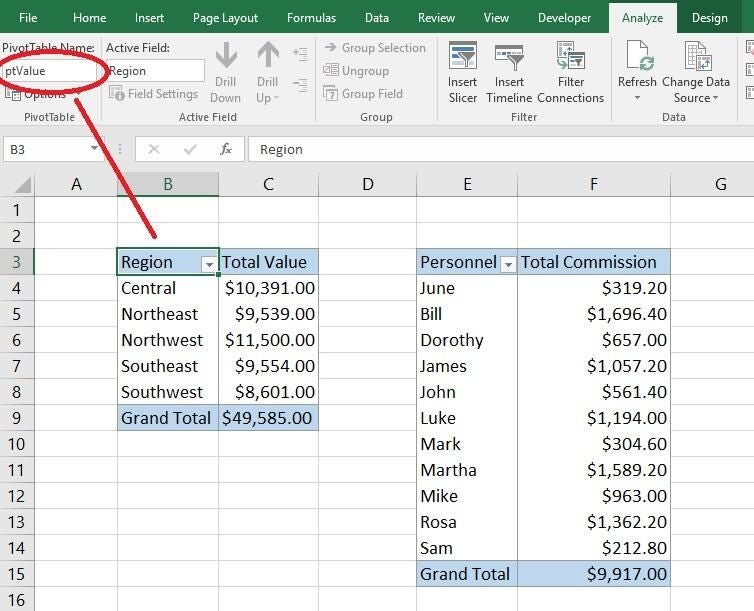
Name the PivotTable ptValue.
Add and connect the slicer
Now we’re ready to add the slicer that will filter both PivotTables at the same time. To get started, select ptValue (although you could click either) and then do the following:
- Click Insert Slicer in the Filter group (on the contextual Analyze tab).
- In the resulting dialog, check Region (Figure F).
- Click OK.
- Drag the slicer to locate it in a convenient spot.
Figure F
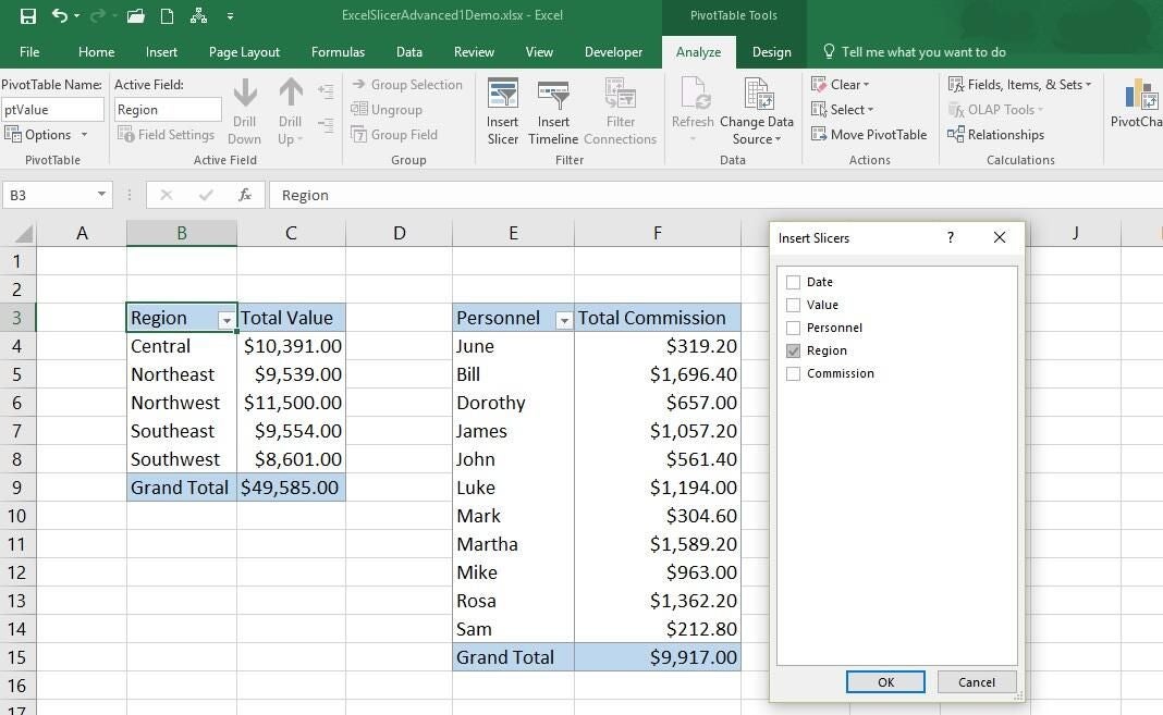
Choose a filtering column.
Right now the slicer is connected to only one PivotTable–the one you selected. Clicking any region in the slicer will update only ptValue. To add the second PivotTable, ptCommission, do the following:
- Right-click the slicer and choose Report Connections (Figure G). If you’re using an earlier version, look for PivotTable Connections. The resulting dialog will show the possible connections and the current connection, ptValue, will be checked.
- Check ptCommission (Figure H) and click OK. Now, when you click a region in the slicer, both PivotTables respond, as shown in Figure I. Clicking shows the total for that region in ptValue and the commission for each person who has sales for that region in ptCommission. Remember earlier when I had you name the two PivotTables? This step is why. If you have two PivotTables to work with, as in this example, you won’t have any problem knowing which to check. If you have several PivotTables, which is likely, meaningful names takes the guesswork out of this step.
Figure G
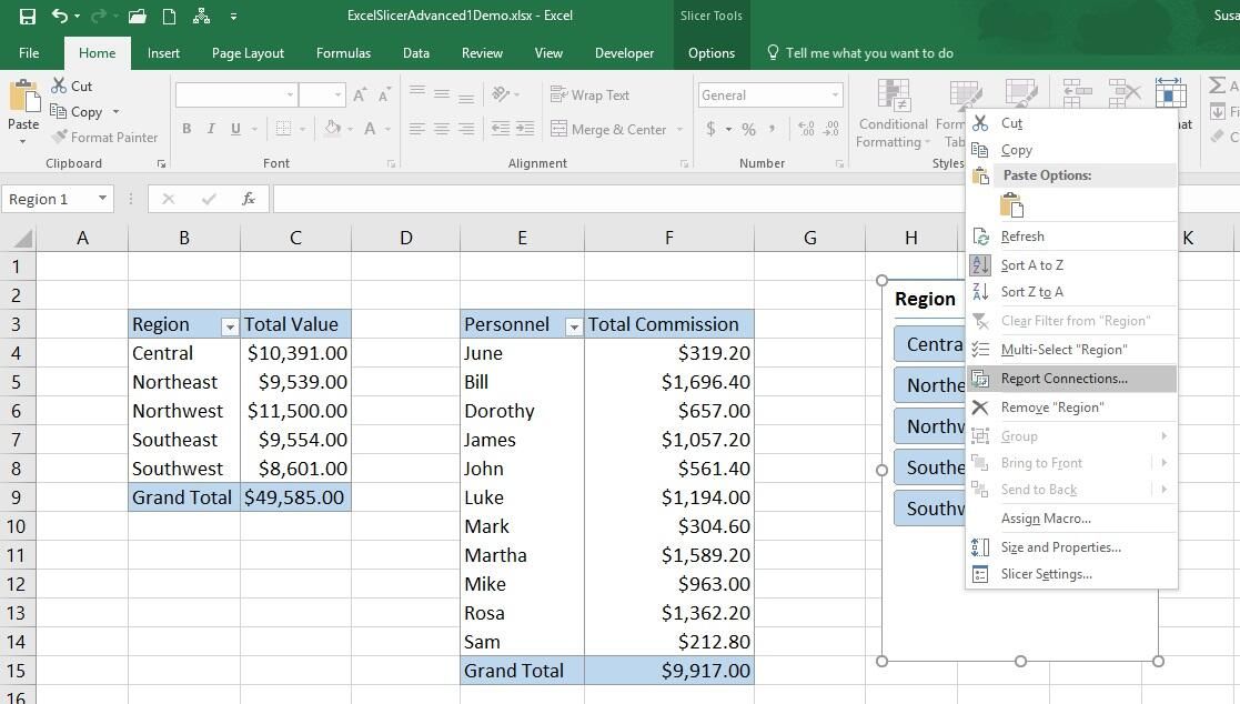
Access the connections.
Figure H
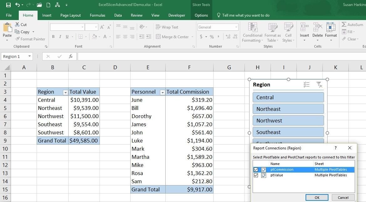
Check all the PivotTable connections that apply.
Figure I
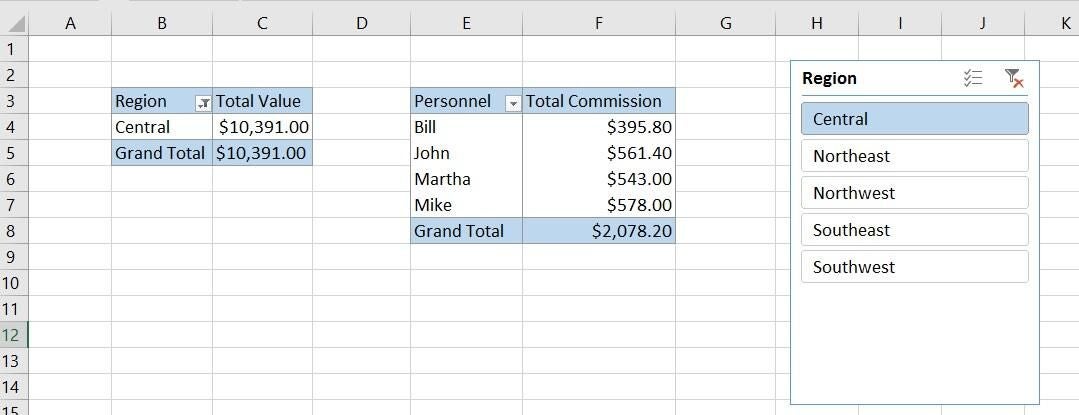
Update both PivotTables.
Format the charts and sheet
Strictly speaking, you don’t have to format the sheet and PivotTables, but you’ll probably want to. Figure J shows the result of doing the following:
- Applying a built-in style to both PivotTables using the contextual Design tab. If the style doesn’t apply the Currency format appropriately, you might need to do so manually.
- Inserting a column to the left of ptValue to improve the placement. (I did this several steps ago but didn’t mention it.)
- Reducing the width of columns D and G.
- Hiding the formula bar, headings, and gridlines; use the View tab to toggle these display options.
- Hiding the Ribbon by double-clicking any tab.
Figure J
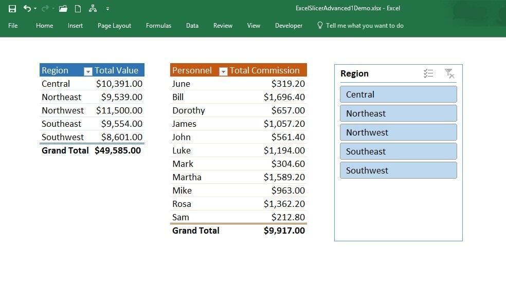
Formatting the sheet and PivotTables removes distractions and looks a bit like a dashboard app.
You can use the slicer as you would any other but remember that it adjusts both PivotTables. You can add more PivotTables to the mix as long as you copy one of the connected PivotTables to create the new one. Any PivotCharts you create from these PivotTables will also be linked to the slicer. There’s a connected PivotChart in the downloadable demo file, although, I don’t offer instructions–you won’t need them.
Send me your question about Office
I answer readers’ questions when I can, but there’s no guarantee. Don’t send files unless requested; initial requests for help that arrive with attached files will be deleted unread. You can send screenshots of your data to help clarify your question. When contacting me, be as specific as possible. For example, “Please troubleshoot my workbook and fix what’s wrong” probably won’t get a response, but “Can you tell me why this formula isn’t returning the expected results?” might. Please mention the app and version that you’re using. I’m not reimbursed by TechRepublic for my time or expertise when helping readers, nor do I ask for a fee from readers I help. You can contact me at susansalesharkins@gmail.com.