


Must-read Windows coverage
- CrowdStrike Outage Disrupts Microsoft Systems Worldwide
- 10 Best Project Management Software for Windows in 2024
- Windows 10 Extended Security Updates Promised for Small Businesses and Home Users
- Securing Windows Policy
If you’re working on your accounts and you need to convert all your overseas expenses into the currency you file your tax returns in, you need to know the exchange rate for the date of every expense. You don’t have to fill that in by hand: you can get a list with the daily exchange rates and get Excel to look up the right conversion for every expense. You can also use VLOOKUP when you need to find a part by the part number, an employee by their employee number, the international dialling code for a country, or anything else that you look up by a key from a master record that doesn’t make sense to copy into your current spreadsheet.
But if you only do that once a year, you’ll probably have to research how to use the VLOOKUP function in Excel.
For the third most used function in Excel (after SUM and AVERAGE), VLOOKUP is complex. By default it finds approximate matches, although that’s hardly ever what you want, so you need to remember to set FALSE in the function. And it’s not flexible: if you add or delete a column in the sheet where you’re looking figures up, the formula doesn’t get updated the way it does for functions like SUM, so you have to change your VLOOKUP formula by hand. You have to arrange the source data so the index column, like the date, is on the left and the values you want, like the rate, is on the right; you can’t find the day when the exchange was worst or best without having a second copy of the data with the data in a different order. You can’t change the search order, and if you need to look up information that’s in rows rather than columns you have to use a different function, HLOOKUP, instead.
VLOOKUP can also be a performance hit because it creates an array covering the index column, the column with the data you need and any other columns in between them — even though you don’t care about the data in between.
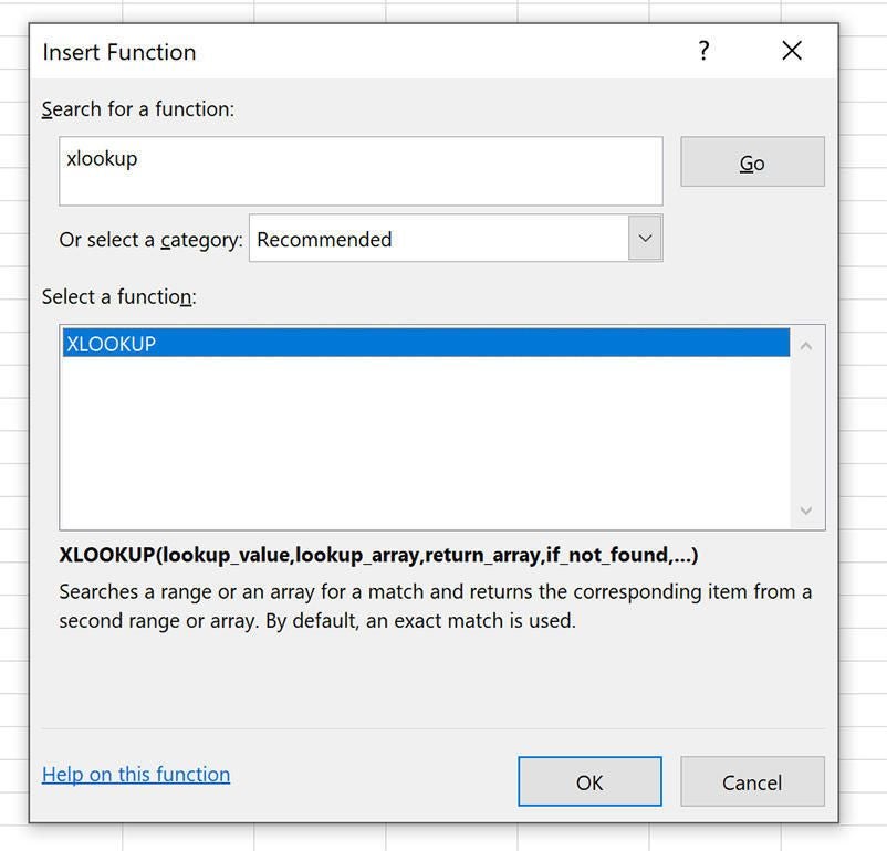
Image: Mary Branscombe/TechRepublic
The new XLOOKUP function fixes all those problems, as it’s simpler, more flexible and won’t slow your spreadsheets down the same way. You can look up results from rows or columns, and the column of data doesn’t have to be on the right of the index column. You can point XLOOKUP at multiple columns and retrieve more than one piece of information — you could look up both the employee name and the department they’re in, for example. You can include a custom error to fill in (like ‘name not found’) if a match isn’t found instead of getting the default #N/A. You can customise both the search order and how matching works. And the result you get back is a reference, not a value, which means you can pass it into another formula.
XLOOKUP needs at least three parameters: the term you’re using to do the lookup, where to look for the term and the data you need to retrieve for it, and where to put the data that gets looked up.
The first term, lookup_value, can be a cell with the value you’re looking up, a value you type into the formula like a name, or another formula like a calculation. That’s the same as with VLOOKUP, but it can also be a concatenation of multiple cells in an array — B1 & B2 & B3 looks for the value where all three cells match, for example — instead of just a single cell to match on.
But instead of an array like A2:D400 that tells VLOOKUP to look in cells A2 to A400 for the lookup term and then retrieve the value from the same row in column D, XLOOKUP uses two parameters — lookup_array and return_array. For the same lookup, that would be A2:A400 and D2:D400. Instead of creating an array with nearly 1600 cells in, XLOOKUP only has to handle just under 800. The bigger the spreadsheet you’re looking up from, the bigger the performance difference that makes.
Plus if you insert a new column in between the index column and the one the results are in, the formula gets updated automatically instead of breaking the way it would with VLOOKUP — because you’d be getting results back from the wrong column.
If you want to look at multiple columns for the matching value, join them using & — C2:C200 & E2:E200.
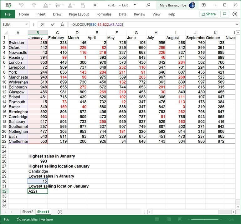
If you need to find out which location had the highest sales, who is using the most of their disk quota or who has used the fewest vacation days, use a MAX or MIN formula in the lookup_value. This is more flexible than it was with VLOOKUP because you don’t have to rearrange the data so the value you’re using to look up information with is always in the leftmost column; XLOOKUP can look left or right, up or down — you just specify which columns or rows to look in.
If you’re looking at those figures in the same spreadsheet, you could just use the total row of a table and set the total to be MAX or MIN or use conditional formatting to pull out information. But if you want to retrieve that minimum or maximum to use in another spreadsheet, you need a lookup function.
If you want to look up multiple pieces of information with the same search you can still use an array, but you can retrieve everything with a single lookup rather than needing one for each piece of information you want to get back. So to look for the employee name in column C and their department in column D, you’d fill in the return_array as C2:D400.
If you’re happy with the standard search order and error, that’s all you need to do your lookup. It’s an easier formula to understand than VLOOKUP. But you can also customise the lookup.
If you want a custom error like ‘name not found’ or ‘no exchange rate for this date’ or something that explains more clearly than #N/A that there wasn’t a match to bring back, put that in quotes as the fourth parameter (which is called [if_not_found]).
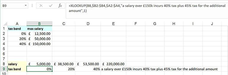
Usually, you’re looking up the exact answer — a name or the exchange rate for a specific day, for example. But you can also look up where on a scale a number falls, like finding what tax bracket a salary falls in. In that case you might not be able to get an exact match. Set the fifth parameter [match_mode] to 1 and if there isn’t an exact match you will get the next largest result; -1 fetches the next smallest item. If you’re matching a salary that falls inside a tax band, you want to match the next largest result because tax bands apply up to a maximum figure. So a salary of £30,000 should look up the tax rate of 20% which applies up to £50,000: matching on the next largest result will get that.
SEE: How to become a developer: A cheat sheet (TechRepublic)
Set the match_mode to 2 and you can use the usual Excel ? and * wildcards to specify what to match on. That way you can search for South and Southeast with ‘South*’ or Northwest and Southwest with ‘*west’.
The default search for XLOOKUP is top to bottom: set the sixth parameter [search_mode] to -1 if you want to search from the bottom of the list until you find the first match.
Function to function
You can nest XLOOKUP functions to pull out a cell from a table by looking up the labels in the top row and left column: use the first XLOOKUP to find the first label and fill in another XLOOKUP function as the return_array to find the second label and the result will be the contents of the cell where they intersect. (That’s like using the INDEX and MATCH functions but you don’t need to learn two more functions.) The easiest way to do it is to have the same labels above and beside the cell where you want to see the result and to use those labels to match on.
The result that comes back from XLOOKUP is a reference to a cell rather than a copy of the value in it, so you can also pass that into another formula. If you do two XLOOKUPs, you can turn that into an array and use SUM to add up all the cells between them, or MAX to find the largest values between the two. That way you could look up the exchange rate at the beginning and end of the month and show the highest rate.
XLOOKUP is currently still in beta; you can only get it if you’re enrolled in the Office Insiders programme. Microsoft has been flighting XLOOKUP to all Insiders since early September, but it may not have reached everyone yet so keep checking if you don’t see it. If you’re using it already, be aware that it may change before it ships as a final feature. Since XLOOKUP was first introduced, the [not_found] parameter was added (it was originally the sixth parameter but then moved to be the fourth parameter so you didn’t have to put in empty parameters to use it).
When it does ship, it will be available as part of an Office 365 subscription and then in the next permanent version of Excel that’s released. So if you’ve already bought a permanent licence to Excel 2019 you won’t get it until you upgrade, the same as with any other subscription feature. If you want to always have the newest Office features as soon as possible, that’s what the Office 365 subscriptions are for.