How to use a conditional format to highlight subtotal rows in Excel

Excel’s Subtotal feature is a great way to quickly analyze data without disturbing the existing structure, because the results are temporary. Unfortunately, the resulting subtotaling rows aren’t well defined when viewed with the detail records. In a large data set, they can be hard to spot. In this article, I’ll show you how to apply a conditional formatting rule that highlights subtotaling rows. When you remove the rows, the format also disappears.

I’m using Excel 2016 on a Windows 10 64-bit system, but this technique will work in older versions. You can work with your own data or download the demonstration .xlsx file. You can’t use Subtotal with a Table object, so when applying this technique to your own work be sure to convert the Table to a range beforehand.

SEE: How to avoid and overcome presentation glitches (TechRepublic PDF)

Without conditional formatting

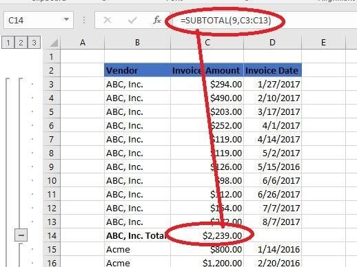
You can work with most any data set, but Figure A shows several rows of invoice vendors, amounts, and dates. We’ll use Excel’s Subtotal feature to display subtotals for the different vendors.

Figure A

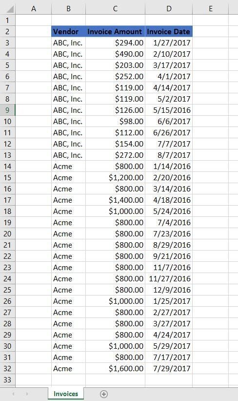
We’ll use Subtotal with this data set.

To generate the subtotals, click anywhere inside the data set and do the following:

Click the Data tab.
Click Subtotal in the Outline group.
In the resulting dialog, choose Vendor from the At Each Change In dropdown, choose Sum from the Use Function dropdown, and check Invoice Amount in the Add Subtotal To list (Figure B).
Check the Replace Current Subtotals and Summary Below Data options if necessary.
Click OK to see the results shown in Figure C.

Figure B

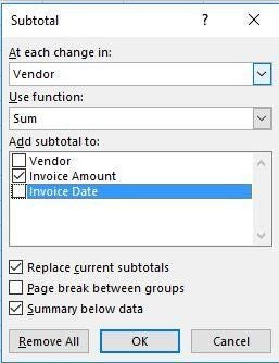
Define the Subtotal options.

Figure C

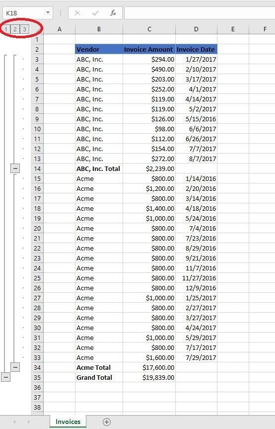
The Subtotal feature adds three subtotaling rows: one for each vendor and a grand total at the bottom.

For better or worse, the feature doesn’t highlight the subtotaling rows. The bold titles are helpful, but they’re not enough. You can click the 2 level button (to the left) to see only the subtotals as shown in Figure D, but that won’t always be adequate.

Figure D

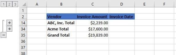
Display only the subtotals.

Our example is simple, but this feature has lots to offer. To learn more about the Subtotal feature, read 10+ tips for working with Excel’s Subtotal feature.

With conditional formatting

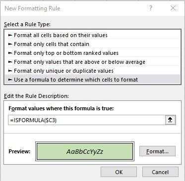
Fortunately, you can add a conditional format to make those subtotaling rows pop. You’ll need a condition though, and there’s no silver bullet. In this case, we can use the ISFORMULA() function because the Subtotal feature adds a SUBTOTAL() function to the subtotaling row, as shown in Figure E.

Figure E

Subtotal adds a function to the subtotaling row.

Before you can set the conditional format, remove the subtotaling rows by clicking Subtotal (Data tab) and clicking Remove All. Assuming you want the entire row formatted, select the data set, B3:D32, and then do the following:

Click the Home tab.
Choose New Rule from the Conditional Formatting dropdown (in the Styles group).
In the resulting dialog, choose Use A Formula To Determine Which Cells To Format in the top pane.
Enter the following formula in the Format Values Where This Formula Is True control:
=ISFORMULA($C3)
Click Format.
At this point, you can use any of the available formatting options. For this example, click the Font tab and choose Italic in the Font Style list. Then, click the Border tab and check the Outline option in the Presets section. Finally, click Fill and choose Green.
Click OK. Figure F shows the formula and the format.
Click OK to return to the sheet.

Figure F

This conditional format will highlight the subtotaling rows.

Currently, the data set contains no formulas in column C so there’s no formatting. Now, using the steps in the previous section, enable Subtotals. As you can see in Figure G, the subtotaling rows jump right out at you! When you remove the subtotals, the formatting disappears.

Figure G

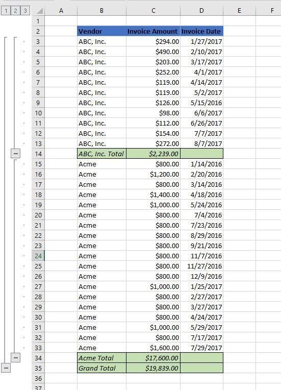
The conditional format rule highlights only subtotaling rows.

Remember earlier when I said there’s no silver bullet? When choosing a condition, you must consider your data. If C3:C32 contained any formulas, this wouldn’t work.

Variations

When applying this conditional formatting solution to your own work, you’ll have different needs. If you want to highlight a single cell in the subtotaling rows, select only the single column before applying the conditional format. You could even add a second conditional formatting rule. For instance, you might want the blank cells in column D to be black. In this case, you’d select B3:C32 to apply the first format and then select column D to apply the second. The conditional formatting rule would be the same. In addition, if the ISFORMULA() function won’t work for you because the column contains formulas other than Subtotal’s SUBTOTAL(), try another condition. You could use =Right($B1,5)=”Total” to find the word Total in the title text (in column B). If someone changes the text, the rule won’t work, so be careful when choosing your condition.

Send me your question about Office

I answer readers’ questions when I can, but there’s no guarantee. Don’t send files unless requested; initial requests for help that arrive with attached files will be deleted unread. You can send screenshots of your data to help clarify your question. When contacting me, be as specific as possible. For example, “Please troubleshoot my workbook and fix what’s wrong” probably won’t get a response, but “Can you tell me why this formula isn’t returning the expected results?” might. Please mention the app and version that you’re using. I’m not reimbursed by TechRepublic for my time or expertise when helping readers, nor do I ask for a fee from readers I help. You can contact me at susansalesharkins@gmail.com.

How to use a conditional format to highlight subtotal rows in Excel

SEE: How to avoid and overcome presentation glitches (TechRepublic PDF)