


Lookup functions are great for finding values that match another value. Thanks to XLOOKUP() this task is easier than ever, and it even supports wildcards! In this article, I’ll show you how to use the asterisk wildcard (*) to create a more flexible lookup value. Instead of finding an exact or almost match, dropping in a wildcard allows you to work with a simpler search string. This setup is helpful when you remember part of the search string, but not all of it. In this article, I’ll show you how to use a wildcard in the XOOKUP() function’s criteria argument, or search string.
SEE: Software Installation Policy (TechRepublic)
Must-read Windows coverage
- CrowdStrike Outage Disrupts Microsoft Systems Worldwide
- 10 Best Project Management Software for Windows in 2024
- Windows 10 Extended Security Updates Promised for Small Businesses and Home Users
- Securing Windows Policy
You could use VLOOKUP(), keeping a few things in mind: You must restructure the source data because the return value is to the left of the lookup value, and VLOOKUP() can’t handle that. I’m using XLOOKUP() going forward though. Unless I run into a specific reason to use one of the older lookup functions, I see no advantage to using them. If you’d like to learn about XLOOKUP(), read How to use the newish XLOOKUP() dynamic array function in Excel.
I’m using Microsoft 365 on a Windows 10 64-bit system. Excel’s XLOOKUP() function is available in Microsoft 365 and Excel 2021, and Excel for the web. For your convenience, you can download the demonstration .xlsx files. This article assumes that you have basic Excel skills, but even a beginner should be able to follow the instructions to success.
Setting things up
Let’s suppose that you use Excel to track products for a gourmet food distributor. As you can see in Figure A, the product names are a bit complex, and it might be difficult to remember them exactly. When searching, you might consider filtering or supplying a data validation control, but in both cases, the product list is long and a bit awkward to work with. The next step might be to use XLOOKUP(), which returns a single value based on a lookup value—in this case, the product names as follows:
=XLOOKUP($I$2,Table2[ProductName],Table2[UnitPrice])
=XLOOKUP($I$2,$D$3:$D$47, $C$3:$C$47)
You must enter the full product name. For instance, if you try to find “Uncle Bob’s Organic Dried Pears” by entering only Pears you’ll be disappointed (Figure A). (Remember, if you’re not using a Table object, your references won’t look the same because Table objects use structure referencing.)
Figure A
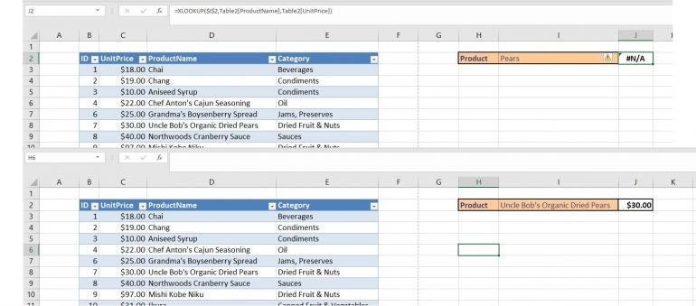
The error value is a good clue; #N/A means the function can’t find the value in I2. If you see a #VALUE error, something’s wrong with the function itself. If you paste the value from column D into I2, the function works as expected, so you know it’s the input value and not the function. There’s no mystery involved. XLOOKUP() wants an exact match, and the current setup can’t get the job done. However, throwing a wildcard into the mix can!
How to add a wildcard in Excel
Don’t worry if you’re not familiar with wildcards, but they are something you should review because they really come in handy. We’ll be using the asterisk character (*), which finds any number of characters. For example, to find the entire product name using only pears as a lookup value, you’d use *pears* as the search string.
You can’t just plug in the asterisk character though. When adding wildcards to a function in this way, you must concatenate the delimiter and the reference. Within this context, concatenation means to combine elements that Excel evaluates into one string and delimiter is a character that helps in the process by identifying the data type. We’ll use the dollar sign character ($) to combine elements.
Now, let’s look back at the original XLOOKUP()
=XLOOKUP($I$2,Table2[ProductName],Table2[UnitPrice])
$I$2 identifies the lookup value, Table2[ProductName] is the column the lookup value needs to match, and Table2[UnitPrice] is the return value when a match is found. In plain English, this function returns the value from the UnitPrice column where the ProductName value matches the value in I2.
The only modification we need to make is to the lookup value, $I$4. Specifically, we need to add two wildcards and use the double quotation characters as string delimiters
"*" & $I$4 & "*"
which evaluate to *$!I$4*. The string delimiters around the asterisk characters are required. The modified function
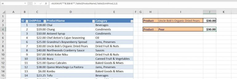
=XLOOKUP("*"& $I$4 &"*",Table2[ProductName],Table2[UnitPrice],2,2)
handles the wildcard correctly, as shown in Figure B.
=XLOOKUP("*"& $I$4 &"*",Table2[ProductName],Table2[UnitPrice],2,2)
Figure B
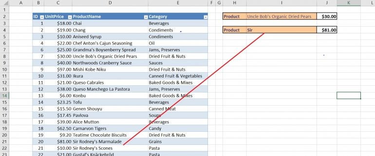
The one thing I want to point out is that this function returns a single value. Try entering Sir into I4. As you can see in Figure C, the function returns $81, matching Sir Rodneys’ Marmalade in D21. Do you see the problem? The value in D22 also contains the string Sir. This is the one hitch that might be a problem.
Figure C
A warning about duplicates in Excel
When using XLOOKUP() to find a single value, you can use a wildcard as shown, but the possibility exists that the function might not return the right value if the search string exists in more than one value. For this reason, you might want to alert the user that other matching records exist.
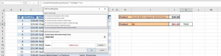
We can approach this alert in a number of different ways, but the simplest method is to use conditional formatting. In this case, we need to alert the user when the search string matches two or more records. First, we need to decide what to highlight: The results in J4 or the actual products. You could do either or do both. We’ll do the former using the following expression
=COUNTIF(Table2[ProductName],"*" & $I$4& "*")>1
in cell K4. This function returns TRUE if the search string (currently Sir) occurs more than once in the ProductName column and FALSE if not. If you prefer that users not see this helper function, reduce the column width or even hide the column (I don’t really recommend the latter because functions are easy to forget and find later.) Now you’re ready to create the conditional formatting rule:
- Select I4:J4. On the Home tab, click Conditional Formatting in the Styles group and choose New Rule from the resulting dropdown.
- In the top pane of the resulting dialog, click Use a Formula to Determine Which Cells to Format the control in the bottom pane, enter
=$K$4=TRUE - Click Format.
- Click the Font tab, choose a bright eye-catching color, such as red from the Color dropdown, and then click OK. Figure D shows the function and the format.
- Click OK to return to the sheet. Notice that the rule uses the red font for Sir and $81 because the search string, Sir, occurs more than one in the ProductName column.
Figure D
If you’re the only one who uses the sheet, you can stop here. It’s unlikely you’ll need a reminder as to what the highlight means. At this point, finding the duplicates in the name column is a quick Find task. Simply drop *Sir* into the Find What control.