
Scrolling around a large sheet can be tedious, awkward, and occasionally, even fruitless because you simply can’t find what you’re looking for. Thanks to the Name box in Microsoft Excel, you can arrive at your destination with little effort, regardless of how far away it is. In this tutorial, I’ll show you how to use Microsoft Excel’s Name box to get a lot done without much effort.
SEE: Windows, Linux, and Mac commands everyone needs to know (free PDF) (TechRepublic)
I’m using Microsoft 365 on a Windows 10 64-bit system, but you can use earlier versions. Excel for the web supports the Name box, but GoTo, mentioned in the first section, isn’t available.
What is Excel’s Name box?
Excel’s Name box is a powerful tool for an ordinary dropdown. To find it, look to the left of the Formula bar. Usually, it displays the reference for the current cell as shown in Figure A. The dropdown displays named ranges.
Figure A
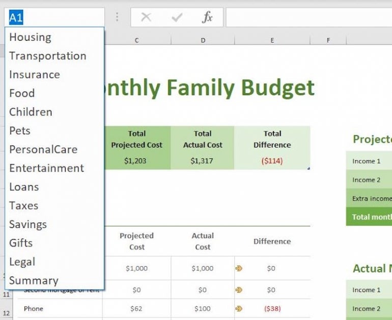
Besides displaying the address of the active cell, Excel’s Name box does much more:
- Name displays the name of the cell, range or object selected.
- Name helps you name a cell, range or object, such as a picture or chart.
- Name lets you quickly access a reference or named range: If you select a range, the box displays the anchor cell, the top-left cell or the bottom-right cell, depending on how you selected the range.
- Name’s dropdown lists named ranges.
The Name box supports a range name’s scope. For instance, all workbook scope-level and current sheet-level range names appear in the dropdown. Sheet-level range names only appear when their sheet is the current sheet. This explains why sometimes you know the range exists, but you don’t see it in the dropdown.
How to use the Name box to select a cell in Excel
Excel’s Name box lets you select cells or ranges by entering a reference or range name. The dropdown shows the range names in the workbook file. Enter a cell reference or select a range name from the dropdown to quickly access that area of the workbook.
Let’s try a quick example:
- Before blasting off, select A1, so you can learn a quick trick about coming back.
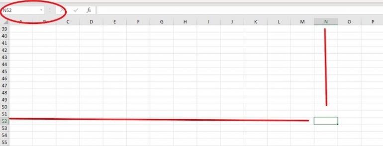
- In the Name box, enter a cell far off screen, say N52, and press Enter. To access a cell on another sheet, be sure to include the sheet name ‘Sheet2’!N52.
- Instantly, the cursor is at N52 (Figure B). Don’t do anything else — not just yet.
Figure B
I promised a quick return to A1, so here it is:
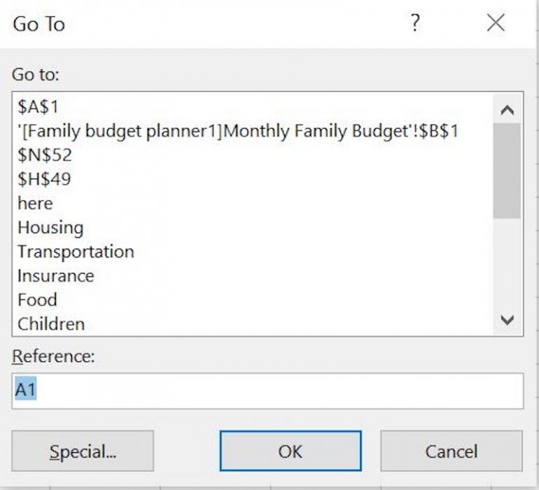
- Press F5. Notice that the cell in the Reference control is A1 (Figure C).
- Press Enter or click OK to quickly return to A1.
Figure C
That’s it — you’re back at A1. This only works once. If you move to N52 and then move around a bit in that area, you will lose the quick route back to A1.
You can select a range the same way. For instance, enter A1:E1 and press Enter. Excel selects that range.
If you enter A1, E1 and press Enter, Excel will select the non-contiguous range of A1 and E1. To select an entire column, such as D, enter D:D. Similarly, to select an entire row, such as 2, enter 2:2. To select multiple columns, such as D and F, enter D:D, F:F. Similarly, to select multiple rows, such as 2and 4, enter 2:2, 4:4. Excel requires the commas.
You can even move between open workbooks by including the workbook name. For instance, to access A1 on Sheet1 in a workbook named Book2, enter [Book2]Sheet1!A1 in the Name box and press Enter — Book2 must be open.
To quickly access the Name box from anywhere in the workbook, press Alt + F3.
You can use the Name box to select a cell, a range or a named range. You can also use Name to create a named range.
How to use Name to create a named range in Excel
On Excel’s Formula tab, the options in the Defined Names group help you name a range. To go to a range, simply select it from the dropdown. You can also use the Name box to name a range and bypass the options on the Formulas tab. To quickly name a range without using any other option but the Name box, do the following:
- Select the range you want to name. For this example, select A1:E1.
- In the Name box, enter NameTest (Figure D), and click Enter.
- Select a cell other than A1:E1.
- Click inside the Name box, enter NameTest, and press Enter. Doing so takes your right back to A1:E1.
Figure D

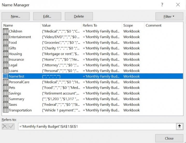
NameTest is now a valid range name. If you like, click Name Manager in the Define Names group. As you can see in Figure E, you now have a range named NameTest at A1:E1. One thing the Name box can’t do for you is rename the range name. Use the Manage Names feature to do that.
Figure E
When using the Name box to name ranges, you must obey the same rules as you would using the Define Names options:
- Don’t use spaces or punctuation: You can use the underscore (_) instead of a space to improve readability.
- Names are case sensitive.
- Start the name with a letter, underscore (_) or backslash (\).
- Names can’t exceed 255 characters.
So far, we’ve used the Name box to move around and create named ranges. You can also access functions.
How to use Name for quick access to common functions in Excel
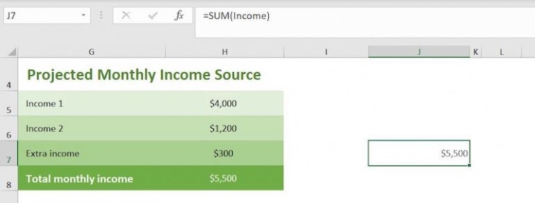
Excel’s Name box automatically lists common functions in the dropdown when you enter the equals sign. From that dropdown, you can click the function you want instead of typing it. To demonstrate, we’ll name a range and then use it in a SUM() function:
- Select H5:H7 — the income values.
- In the Name box, enter Income and press Enter (Figure F).
- Select J7 and enter =.
- Check the Name box; it displays SUM. Select SUM from the Name box dropdown.
- In the resulting dialog, replace the range address with Income (Figure G).
- Click OK and Excel returns the total of the income values in H5:H7 (Figure H).
Figure F

Figure G

Figure H
Excel’s Name box is a powerful tool for moving quickly around a sheet or workbook, and more.


