


Image: muchomor, Getty Images/iStockphoto
Must-read Windows coverage
- CrowdStrike Outage Disrupts Microsoft Systems Worldwide
- 10 Best Project Management Software for Windows in 2024
- Windows 10 Extended Security Updates Promised for Small Businesses and Home Users
- Securing Windows Policy
TechRepublic member Jeff has an interesting and challenging Microsoft Excel problem: He wants to apply a conditional count to the last seven rows of a data set that updates daily–that means the solution has to be dynamic. Right now, he can apply the conditional count, but he has to update the formula every day, which is tedious.. I’ll show you the solution I suggested for Jeff: Use an OFFSET() function to accommodate the changing data range.
I’m using Microsoft Excel in Office 365 desktop on a Windows 10 64-bit system, but this solution will work in older versions and in the browser. You can work with your own data or download the demonstration .xlsx file (the .xls format won’t support this solution).
Why do you need Offset()?
We’ve kept the data set simple: Two columns and a row for every day (Figure A). The status values are the conditional values yes and no. In addition, it’s a Table object.
Figure A
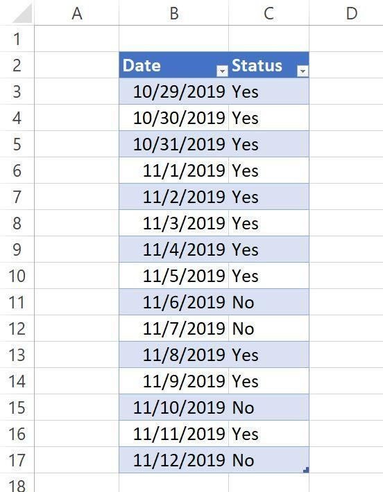
Jeff uses a counting function to return the number of Yes values in the last seven rows. Using cell references, he must update the reference every day to accommodate the new daily record. Jeff needs a dynamic formula that automatically adjusts the data range when a new record is added. For that, we’ll use the Offset() function.
What does Offset() do?
Excel’s Offset() function returns a range specified by a specific number of rows and columns, dependent upon an anchor cell. This function uses the following syntax:
OFFSET(reference, rows, cols, [height], [width])
In a nutshell, you’re building a range:
- reference is the first cell in the data set. In our case, that’s C3—the first status cell.
- rows is the number of rows up or down that you want to reference, based on reference.
- cols is the number of columns to the left or right that you want to reference, based on reference.
- height determines the number of rows you want the returned reference to be. This is an optional argument and must be a positive number.
- width determines the number of columns you want the returned reference to be. This is an optional argument and must be a positive number.
Now, let’s create an Offset() function that Jeff can use, beginning with an input cell so the returned range is dynamic.
How to use the input cell
Jeff wants the returned range to evaluate the last seven rows in the data set. We could enter 7 into the expression, but instead, let’s use an input cell so Jeff can change the size of the returned range on the fly; Jeff doesn’t need this flexibility, but you might. Figure B shows the new input cell. E3 is a named range, n_rows. (Select E3 and enter n_rows in the Name Box.)
Figure B

With the input cell in place, you’re ready for the expression that does the counting.
How to write the expression
The expression we’re going to use combines CountIf() and Offset(). The Offset() function returns a range that’s evaluated by the CountIf(). Enter the following expression in G3 (Figure C).
=COUNTIF(OFFSET(C3,COUNTA(Table1[Status]),0,-n_rows-1),”Yes”)
Figure C
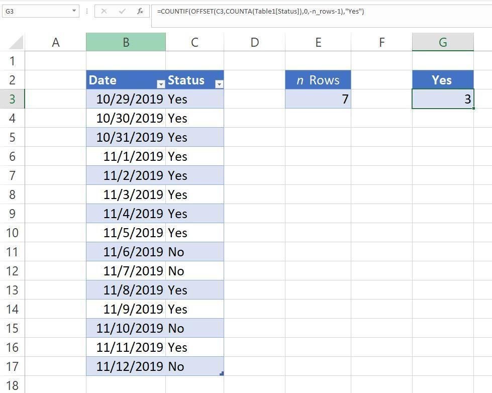
Perhaps the easiest way to explain how this works is to evaluate it in pieces:
- reference is C3 the anchor cell—the upper-left cell.
- rows is the CountA() function, which returns the number of cells in the Status column (15). This value will increase with each new record. The Table[Status] reference could be a traditional cell reference, but we need the Table object’s dynamic properties to make this technique work.
- cols is 0 because the counting takes place in the Status column; we don’t need to expand the returned range by any columns.
- height is -n_rows-1, the input cell minus 1, which returns 6.
- width isn’t necessary because we’re not expanding the columns.
Now let’s put it all together to see how it works.
=COUNTIF(OFFSET(C3,COUNTA(Table1[Status]),0,-n_rows-1),”Yes”)
=COUNTIF(OFFSET(C3,15,0,6), “Yes”)
=COUNTIF(C11:C17, “Yes”)
=3
The total number of cells is 15, and the returned range starts nine rows down from there at C11: 15-(7-1) = 9. The returned range is C11:C17. This is why the data set must be a Table object—it automatically adjusts the last cell reference as you add new rows. If you were using an ordinary data range, this solution wouldn’t work.
Here’s another input cell to try
Jeff doesn’t need more flexibility, but you might, so let’s add one more input cell: The conditional values Yes and No. For this purpose, we’ll use a validation control.
- Select F3. Click the Data tab and then click Data Validation in the Data Tools group. If necessary, choose Data Validation from the dropdown.
- In the resulting dialog, choose List from the Allow control and enter Yes,No in the Source list (Figure D).
- Click OK.
Figure D

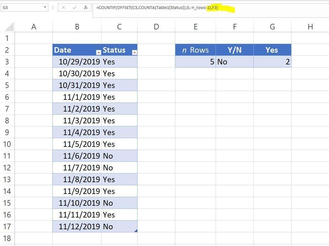
Next, modify the expression to reference the new input cell:
=COUNTIF(OFFSET(C3,COUNTA(Table1[Status]),0,-n_rows-1),F3)
Replace Yes with F3—that’s the only change. Now, you can decide whether the function counts the Yes or No values and determine how many rows will be counted (Figure E).
Figure E
You’ll notice that I didn’t use a named range for F3 as I did for E3. It works both ways—you can use the actual reference or use a named range for both input cells. There are good reasons for using named ranges, but in this case, it doesn’t matter. You might run into a situation where a named range offers more flexibility than a cell reference.
If you have another solution for Jeff, please share your ideas in the comments section below.
Send me your question about Office
I answer readers’ questions when I can, but there’s no guarantee. Don’t send files unless requested; initial requests for help that arrive with attached files will be deleted unread. You can send screenshots of your data to help clarify your question. When contacting me, be as specific as possible. For example, “Please troubleshoot my workbook and fix what’s wrong” probably won’t get a response, but “Can you tell me why this formula isn’t returning the expected results?” might. Please mention the app and version that you’re using. I’m not reimbursed by TechRepublic for my time or expertise when helping readers, nor do I ask for a fee from readers I help. You can contact me at susansalesharkins@gmail.com.