


Excel has built-in tools to expose and even delete duplicates, but they work on existing data after the fact. If you want to make sure duplicates never happen in the first place, you might consider using Excel’s data validation feature. This feature checks values as you enter them and depending on the rules you specify rejects or accepts that value. Unfortunately, there’s no built-in validation rule that recognizes a duplicate value, so you’ll need to combine the feature with Excel’s COUNTIF() function.
In this article, I’ll show you how to do this in a Table object using structured referencing and named ranges.
More about Software
- Software Installation Policy
- Five Methods to Insert a Checkmark Into Microsoft Office Products
- How to Hide and Handle Zero Values in an Excel Chart
- How to Use Section Breaks to Control Formatting in Word
I’m using Office 365’s Excel 2016 (desktop) on a Windows 10 64-bit system, but both techniques will work in earlier versions and in the browser edition. You can work with your own data or download the demonstration .xlsx and .xls files.
SEE: Windows 10 power tips: Secret shortcuts to your favorite settings (Tech Pro Research)
About COUNTIF()
There’s no built-in duplicate rule for Excel’s Data Validation feature, but you can combine the feature with the COUNTIF() function to get the job done. To do so competently, you need to know about the COUNTIF() function. (Feel free to skip this section, if you know how to use this function.)
The COUNTIF() function counts the number of cells in a range that meet a specific condition. You supply the range and a condition as arguments using the following syntax:
COUNTIF(range,condition)
Let’s use this function to count the number of times a membership number occurs within column B, the Membership Number column, of the sheet shown in Figure A. Right now, this column allows duplicates.
Figure A
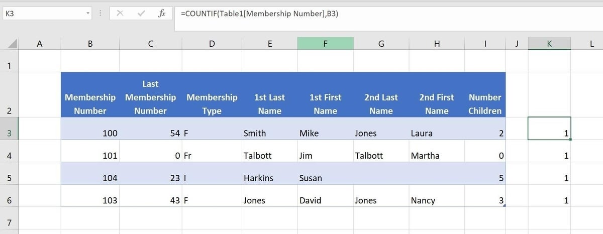
We’ll use data validation to prevent duplicate numbers in the Membership Number column.
First, enter the following function into cell K3:
=COUNTIF(Table1[Membership Number],B3)
The function uses structured referencing because the data is formatted as a Table object. Because the value 100 occurs only one time within the column, the function returns 1. Copy it to the remaining cells to see that they all return 1 (Figure A). If you repeat one of the values, the respective functions return 2, as shown in Figure B. You could use conditional formatting to warn you that a duplicate exists, but wouldn’t it be better to avoid the duplicate altogether?
Figure B
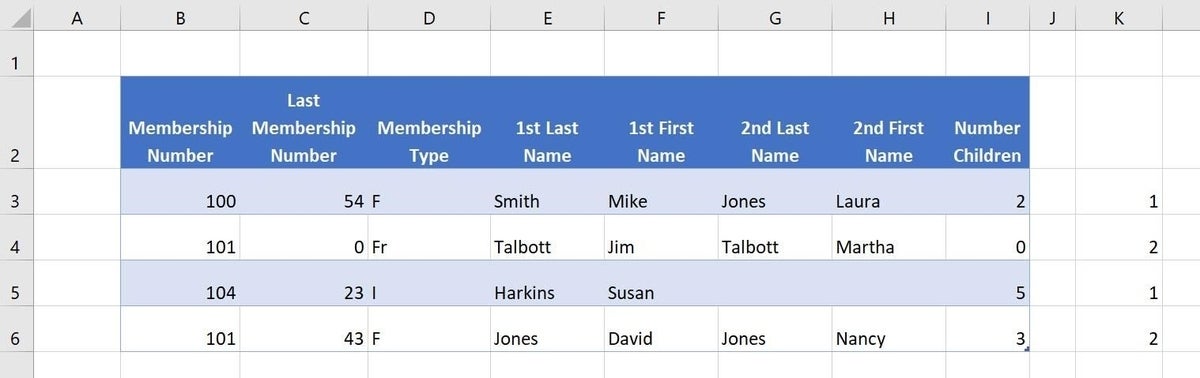
The function returns the number of times the condition is met.
Table accommodations
By adding the COUNTIF() function to the data validation settings, you can use this feature to reject a value if it already exists within range. Before you start, make sure the column in question contains no duplicates. We can illustrate this technique by adding such a validation data control to the Membership Number column as follows:
- Select all existing data cells in the column in question. In this case, that’s B3:B6.
- Click the Data tab, and choose Data Validation from the Data Validation dropdown (in the Data Tools group).
- In the resulting dialog, choose Custom from the Allow drop-down.
- In the Formula control, enter the formula (Figure C)
=COUNTIF(INDIRECT(“Table1[Membership Number]”),B3)<=1
making sure to use straight (not curly quotes). If you’re working with your own data, be sure to update the name of the Table and column. - Click OK.
Figure C
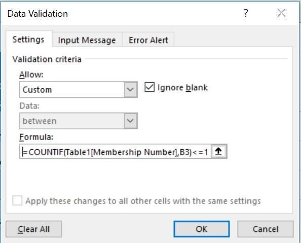
This custom rule will reject duplicates in the Membership Number column.
You don’t have to know exactly how the INDIRECT() function works, but briefly, it returns the reference as text. Without this function, the feature rejects the function because of the structured referencing necessary to accommodate Table objects. (You could enter the actual range, but you’d need to define a name for the range first. I’ll show you how to do that in the next section.)
Thanks to the Table and the INDIRECT() function, range increases every time you add a row. If you enter an existing value in any cell in range, the feature rejects it, as shown in Figure D. The error message isn’t particularly helpful unless you know about the duplicates rule; you can use the feature’s Input Message and Error Alert tabs (see Figure B) to display meaningful information to your users.
Figure D
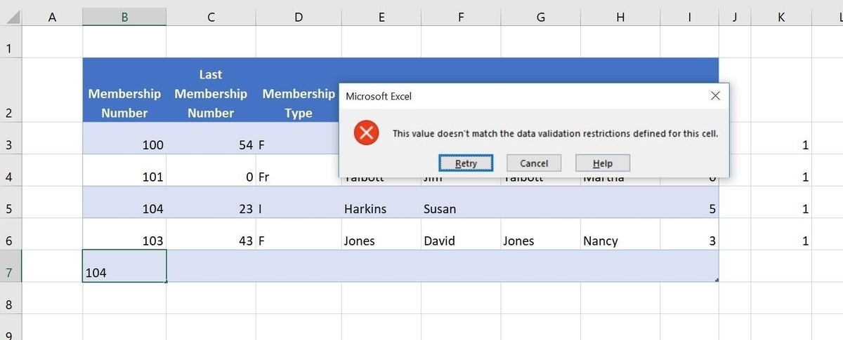
The custom rule rejects a value if it already exists in range.
Named range
There’s no reason to avoid INDIRECT(), but you can use named ranges instead. You can apply a name to the existing data cells as follows:
- Select B3:B6.
- Enter MNumber in the Name control (Figure E).
- Press Enter. You must press Enter to commit the name.
Figure E
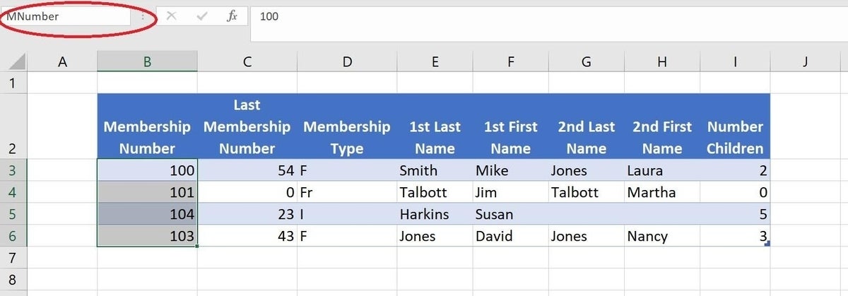
Use the Name control to name a range.
Next, create a validation rule as you did before, but enter the following function, which references the named range instead of using INDIRECT():
=COUNTIF(MNumber,B3)<=1
The two rules work the same, but one works with the Table structure, one works with a named range.
Send me your question about Office
I answer readers’ questions when I can, but there’s no guarantee. Don’t send files unless requested; initial requests for help that arrive with attached files will be deleted unread. You can send screenshots of your data to help clarify your question. When contacting me, be as specific as possible. For example, “Please troubleshoot my workbook and fix what’s wrong” probably won’t get a response, but “Can you tell me why this formula isn’t returning the expected results?” might. Please mention the app and version that you’re using. I’m not reimbursed by TechRepublic for my time or expertise when helping readers, nor do I ask for a fee from readers I help. You can contact me at susansalesharkins@gmail.com.
See also
- A super easy way to generate new records from multi-value columns using Excel Power Query (TechRepublic)
- 3 ways to add glossary terms to a Microsoft Word 2016 document (TechRepublic)
- Excel errors: How Microsoft’s spreadsheet may be hazardous to your health (ZDNet)
- Five tips for using Outlook 2016’s AutoComplete list efficiently (TechRepublic)
- How to use VBA to select an Excel range (TechRepublic)