


When working with a large workbook or a sheet of dozens of columns and hundreds of rows, being able to find specific values quickly is a must-have skill. After reviewing this feature’s basics, I’ll show you how to push this feature a bit further than you might expect it to go. Specifically, I’ll show you how to format and even delete matching values.
More about Software
- Software Installation Policy
- Five Methods to Insert a Checkmark Into Microsoft Office Products
- How to Hide and Handle Zero Values in an Excel Chart
- How to Use Section Breaks to Control Formatting in Word
I’m using Office 365’s (desktop) Excel on a Windows 10 64-bit system, but you can use what you learn with earlier versions. Both the highlighting and deleting tasks rely on this feature’s Find All option, which isn’t supported by the browser. You can work with your own file or download the demonstration .xlsx and .xls files.
SEE: System update policy template download (Tech Pro Research)
Find basics
It’s likely that you’ve explored Excel’s Find feature, but perhaps haven’t had to rely on it for anything beyond a simple find task–that describes many users. Fortunately, the basics are simple.
Before you start a search task, you have a decision to make: Do you want to search the entire workbook or a specific range? When searching a range, select it first. If you want to search the entire workbook, search any cell on the active sheet. Searching for a specific range is more efficient and is always the best choice when appropriate.
You start the process by pressing Ctrl+F to open the Find and Replace dialog. Or, click Find & Select in the Editing group on the Home tab. From the resulting dropdown, you can choose Find or Replace–they’re both tabs in the same dialog.
Find options
Recently, I was asked to “fix” an Excel app that relied heavily on simple find tasks–it just stopped working and the users were at a loss. “It’s broke!” The file wasn’t broke; somehow, an option was changed and Excel was no longer looking for values but values within formulas. This file had no formulas it was a simple data-tracking sheet. Even if the sheet had contained formulas, any search task was going to return unexpected, and erroneous, results. They weren’t getting what they needed but Excel wasn’t broke.
To access options, shown in Figure A, click the Options button. These options will help you fine-tune the task:
- Within lets you determine where you search–the active sheet or the entire workbook. Sheet is the default. You must change this option to search the entire workbook.
- Search determines the search direction (sort of)–by columns or by rows. You won’t miss data by not changing this option, but you might speed things up a bit. By Rows is the default setting.
- Look in lets you limit a search–to formulas, values, or comments. Having the wrong option set can really mess things up, as I mentioned earlier. Formulas (oddly enough) is the default. Use Formulas to quickly update a reference.
- Match case will find only those values that match the case used in the Find what field. Disabled is the default.
- Match entire cell contents will find only those values that match only the characters entered in the Find what field. It’s a great way to find exact matches or similar matches, depending on your setting. Disabled is the default.
- Format lets you search for specific formats. This is extremely handy if you don’t depend on styles; you can use Replace to update formats with a simple search task. Disabled is the default.
Figure A
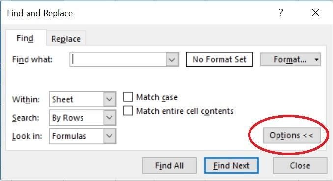
Using the right options is the key to efficient search tasks.
Excel’s Find and Replace feature remembers your settings and that can get you into trouble. Unfortunately, there’s no clear option that resets everything; you must remember to check these options every time you run a search to avoid returning erroneous results.
The basics are easy, and you might be familiar with them already; let’s expand on these basics to run a few search tasks.
Finding values
Knowing what to do with what Excel finds is as important as telling Excel what to find. You have some helpful options: You can view, select, highlight, and even delete matches. Figure B shows the results of opening the Find and Replace dialog, typing in Talbott and clicking Find All. As you can see, the dialog returns a list of every instance of the search string, depending on the options you set. In this example, the options are all the defaults. Let’s review the results within that context.
Figure B
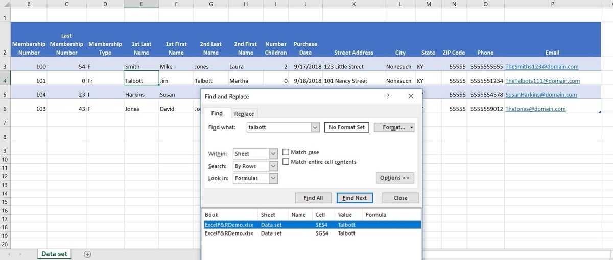
A search string doesn’t always find what you want or expect
The search finds both Talbott entries in row 4. The list would be the same even if either instance of Talbott used a lowercase t–talbott. What might surprise you is that the search doesn’t find the email address because the search string isn’t spelled the same–notice the absence of a second t at the end. Talbott won’t match Talbots. If either of the entries in the name fields were missing that second t, Excel wouldn’t find it either.
To access one of the found items, double-click it in the list. If you click Find Next, Excel moves from one cell to the next instead of displaying a list in the dialog.
Highlighting or deleting matching results
You might never need anything beyond what we’ve reviewed thus far, but there’s more you can do. For instance, using a search task you can highlight and even delete matching entries. To illustrate this, let’s repeat the same search task and then highlight and delete those values (notice that I added the second ending t to the email address).
- Click any cell in the active worksheet and press Ctrl+F to open the Find and Replace dialog.
- In the Find What field, enter Talbott (both ending ts).
- Click Options if necessary and make sure all the options are set to their defaults.
- Click Find All to display the list shown in Figure C. Notice that the feature selects the first matching item in the list. Don’t touch anything else!
- While the selection is active in the resulting list, press Ctrl+A to create a selection of all matched items. Excel also highlights the items at the cell level (although it’s hard to tell with the email address; it’s the last matching value and as such is the active cell, so the selection looks different).
- Once you’ve selected all matching cells, you can highlight the cells by choosing a Fill option in the Font group on the Home tab (Figure D). At this point, you could apply other formats as well.
- Or, right-click any cell in the multi-cell selection and select Clear Contents (Figure E). Of course, I caution you to use great care when doing so. Remember you can press Ctrl+z if you change your mind. (Clicking Delete on the keyboard will delete the list in the dialog, not the matching entries at the sheet level.)
Figure C
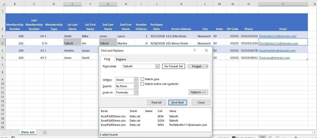
Display all matches.
Figure D
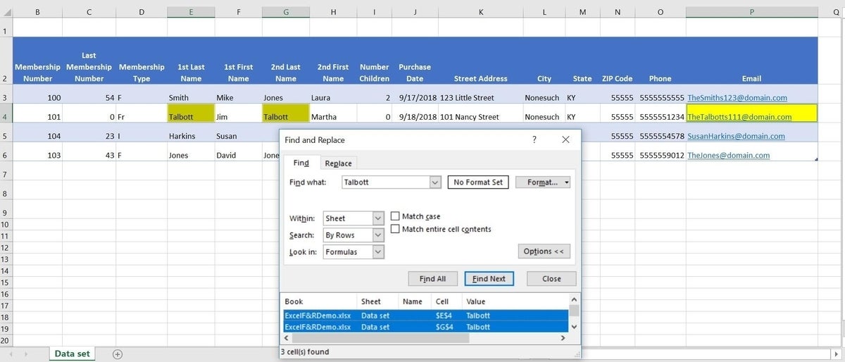
Use a fill color to highlight the matching entries.
Figure E
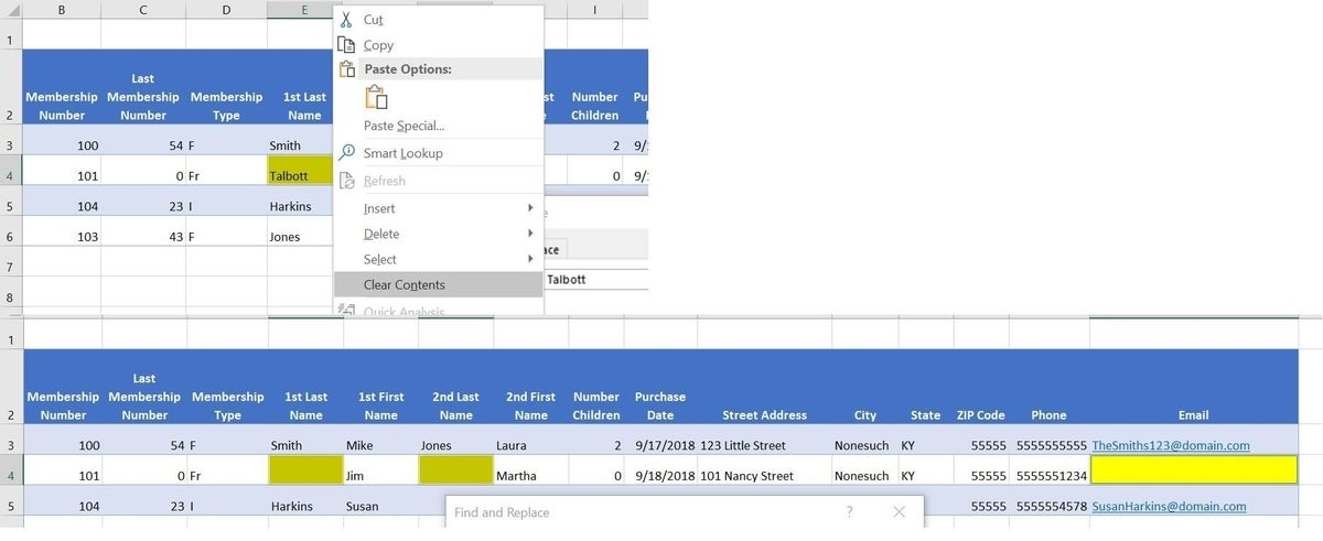
Delete the entries.
Stay tuned
Even if you’re familiar with this feature’s basic purpose, you probably learned how to expand on this feature to apply formats or delete matching values. Next month, we’ll continue with some more advanced techniques.
Send me your question about Office
I answer readers’ questions when I can, but there’s no guarantee. Don’t send files unless requested; initial requests for help that arrive with attached files will be deleted unread. You can send screenshots of your data to help clarify your question. When contacting me, be as specific as possible. For example, “Please troubleshoot my workbook and fix what’s wrong” probably won’t get a response, but “Can you tell me why this formula isn’t returning the expected results?” might. Please mention the app and version that you’re using. I’m not reimbursed by TechRepublic for my time or expertise when helping readers, nor do I ask for a fee from readers I help. You can contact me at susansalesharkins@gmail.com.