How to create two advanced dynamic lists in Excel

The article Five ways to take advantage of Excel list features showed five basic list features built right into Excel. You don’t have to do much to take advantage of them, but sometimes you’ll need something more sophisticated. In this article, I’ll show you two advanced list features using a validation list and a lookup function to generate a dynamic list. Neither technique is superior–your needs will dictate your choice.

I’m using Excel 2016 (desktop), but both techniques will work in earlier versions. For your convenience, you can download the demonstration .xlsx. The VLOOKUP() function is available in earlier menu versions, but both techniques rely on the Table object to be dynamic, and the menu versions don’t support the Table object. The browser edition supports validation lists and Table objects, but inserting new data into a Table is awkward–that edition ignores the Tab wrap to the new record behavior when entering a new record.

SEE: 30 things you should never do in Microsoft Office (free TechRepublic PDF)

A dynamic validation list

A validation list lets you limit users to specific values. You’ll want to use these lists to ease data input and to prevent errors. You can’t keep a user from choosing the wrong value, but at least it’ll be spelled right. And while that may sound silly, a misspelled value returns erroneous results, whether you’re filtering or using complex functions to analyze your data.

In its simplest form, a validation list isn’t dynamic, but combining the feature with the Table object changes that. If both the data set and the list source are Table objects, Excel updates everything as you work.

Figure A shows a simple sheet with two Table objects. We have a data set in columns B through E and a list of unique shelf code values. We’ll add the validation control to column E and use it to enter the appropriate shelf code for each record.

Figure A

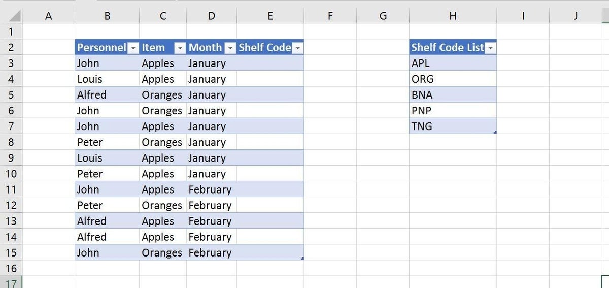
We’ll use these two Table objects to build a dynamic validation list.

These two data sets are Table objects in the demonstration file. If you’re working with your own data, you can convert a data range into a Table as follows:

Click anywhere inside the data set.
Click the Insert tab.
In the Tables group, click Table.
In the resulting dialog, check or uncheck the My Table Has Headers option (Figure B), and click OK.

Figure B

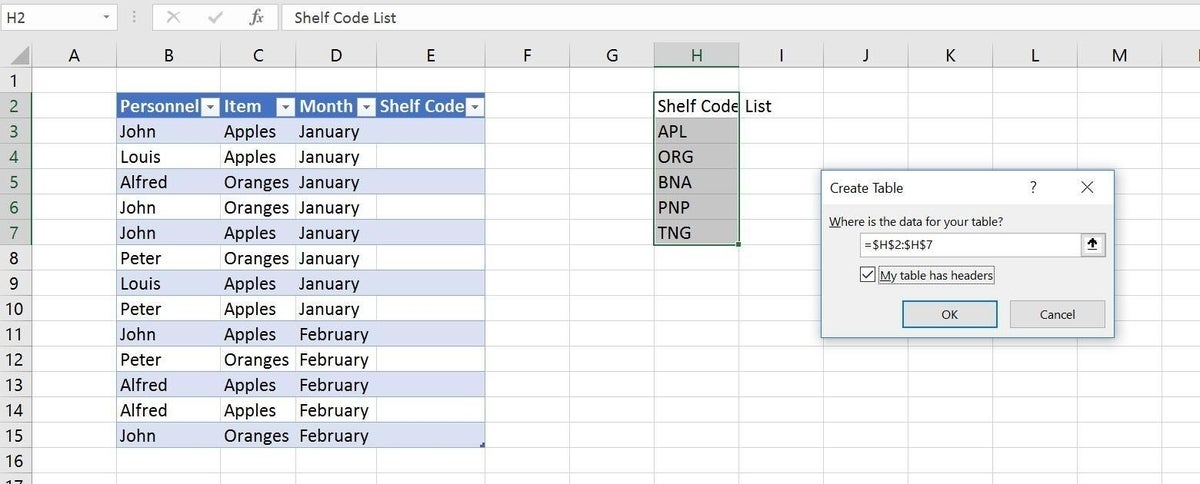
Specify whether your table has headers.

There’s one more step before you can build the validation list. You can’t specify a Table object as the source for a validation list, but you can if you give the Table a range name, as follows:

Select H2:H7 (your list source).
Click the Formulas tab.
In the Defined Names group, click the Create From Selection option.
In the resulting dialog, check Top Row (if necessary), and Excel will use the header text to name the range Shelf_Code_List (Figure C).

Figure C

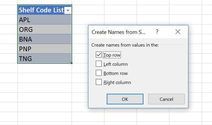
Give the list a range name.

Now you’re ready to create the validation list, as follows:

Select E2:E15–these are the existing cells you want to fill using the validation control. (Your Table might not have any data yet, and in that case, you’ll be selecting a single cell.)
Click the Data tab.
In the Data Tools group, choose Data Validation from the Data Validation dropdown.
From the Allow dropdown, choose List.
In the Source control, enter =Shelf_Code_List, as shown in Figure D. You’re referencing the named range, not the Table object (even though they’re the same range).

Figure D

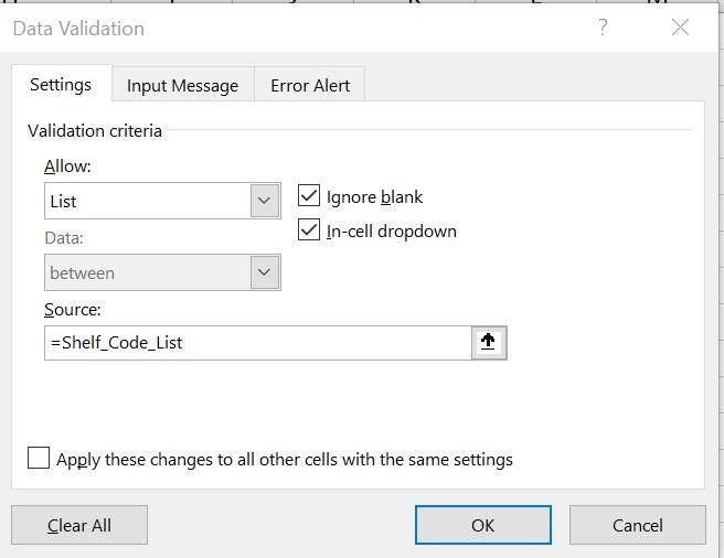
Reference the named range you gave the list source.

With the validation list in place, you can start filling the cells in column E with the appropriate shelf code values. In addition, you can enter each manually by choosing the appropriate code from the dropdown, as shown in Figure E. Once you’ve used a value, just rely on AutoComplete and enter a character or two and let the feature complete the value.

Figure E

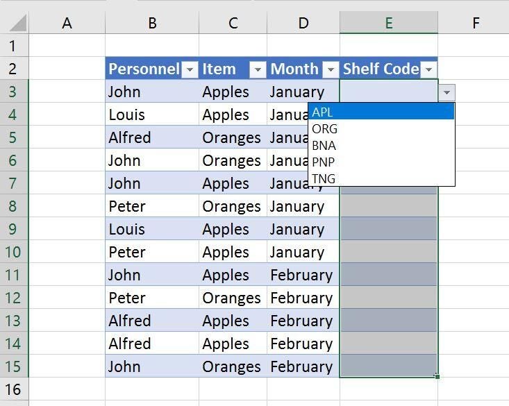
Choose values from the dropdown list.

You might be wondering why the Table objects were necessary. When you add a new record to the Table, Excel extends the validation control automatically (Figure F). You can update the list source and the validation control will update automatically, as shown in Figure G. If you can’t convert the data set into a Table, you must work much harder to get the same dynamic results, but it is possible. You can learn more about a Table-less technique by reading How to use Excel’s Data Validation feature to prevent data entry mistakes.

Figure F

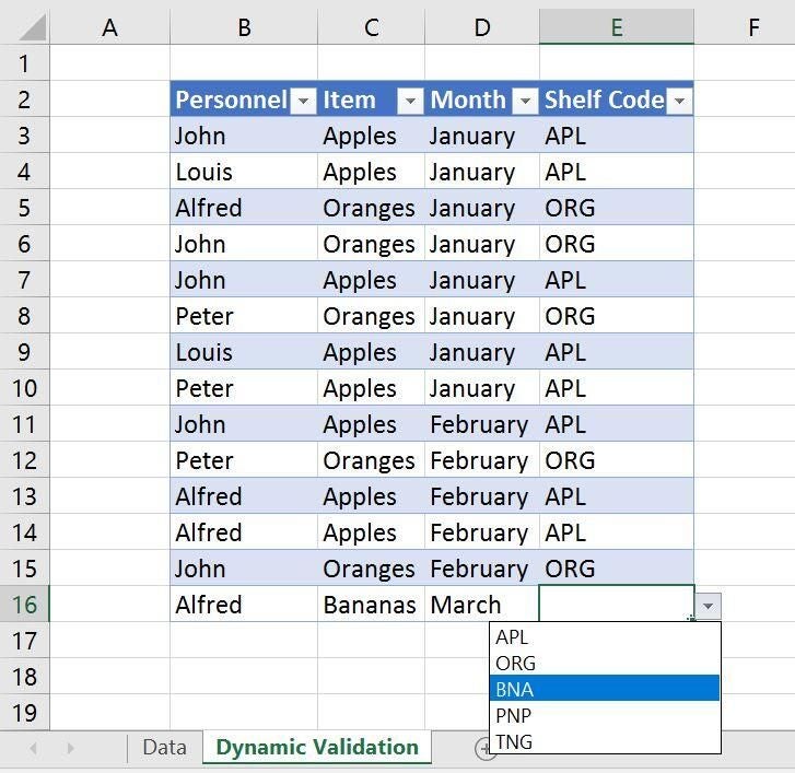
The validation list is available for new records.

Figure G

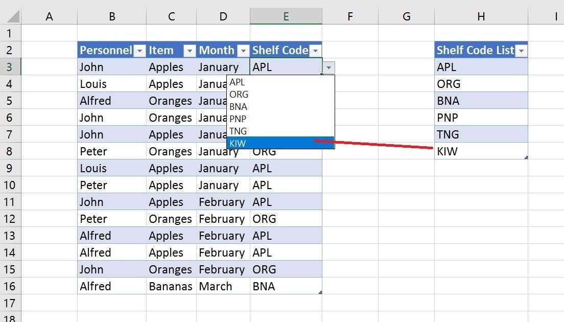
Update the source list.

In such a simple example, an alphabetized list isn’t necessary. If you want an alphabetized list, simply sort the list source, as shown in Figure H.

Figure H

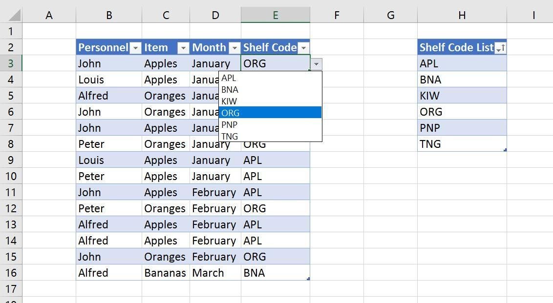
Sort the list source to sort the validation list.

A dynamic lookup function

Using a lookup table, we can negate the task of choosing a shelf code entirely. The downside is that this technique is a bit slow in a complex workbook with thousands of rows. But for most of us, it’ll work fine. It just requires a good understanding of how Excel’s VLOOKUP() function works. Here’s a short tutorial that explains how to troubleshoot VLOOKUP() formula gotchas.

The lookup values require a bit of updating before we can start. As you can see in Figure I, there’s a new Item column to the left of the shelf code column. This is a column of unique values that match the values from the data set. The values to the right–the shelf codes–are the values the function will return when finding a match. For example, when the item value in column C is Apples, the function in column E will return APL.

Figure I

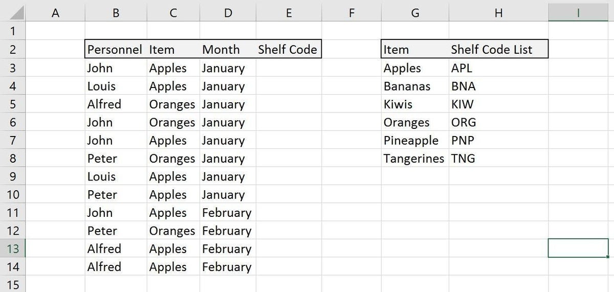
The lookup table needs at least two columns.

To continue, enter the following function in E3 and copy to the remaining data set, as shown in Figure J:

=VLOOKUP(C:C,$G$3:$H$8,2,FALSE)

Figure J

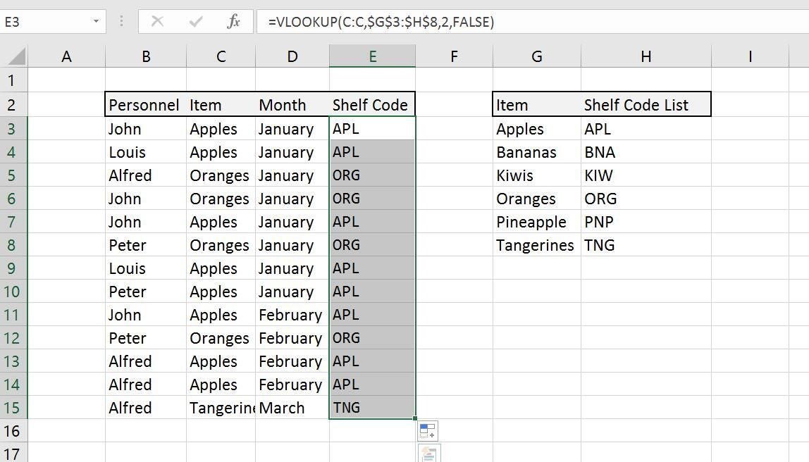
Enter the VLOOKUP() function.

If you enter a new record, as shown in Figure K, Excel extends the formula to the new record. If this doesn’t happen for you, check the following option:

Click the File tab and choose Options.
Choose Advanced in the left pane.
In the Editing Options section, make sure the Extend Data Range Formats And Formulas option is checked (Figure L).
Click OK.

Figure K

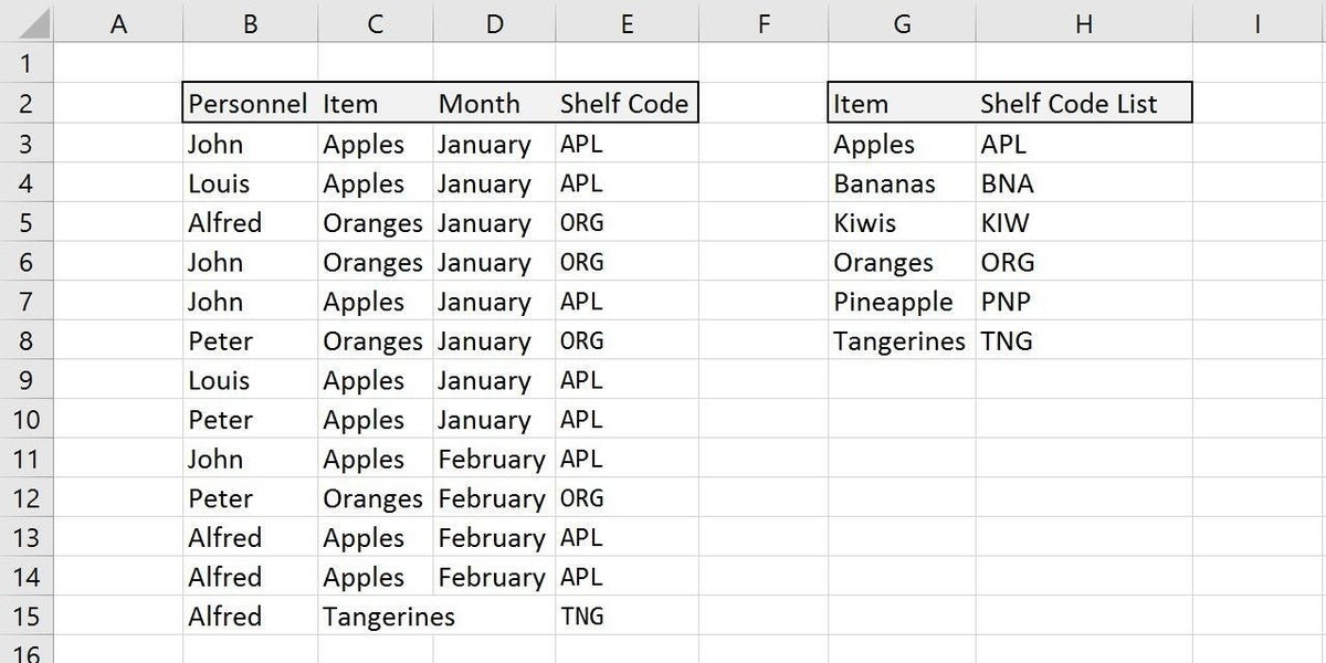
Excel extends the formula.

Figure L

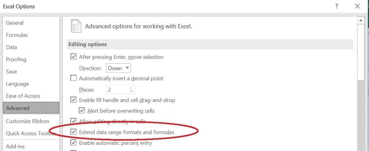
Extend formulas.

As is, the lookup solution isn’t dynamic, so if you add a new fruit to the lookup table (columns G and H), the function in column E won’t update to include that new row. Let’s try that now and see what happens. After adding Coconut; CNT to the lookup table, as shown in Figure M, entering a new record that references Coconut doesn’t update as expected.

Figure M

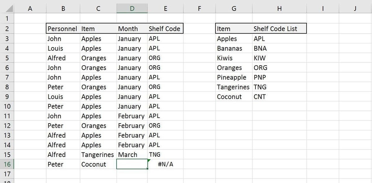
The function doesn’t reference the new lookup item in row 9.

This is where a little Table magic can help. Simply convert the lookup table (G2:H8) to a Table object before you add a new item. Then, add the new item. As you can see in Figure N, the function updates automatically to reference the new row in the lookup Table object. The original function referenced H8, but after converting the data range to a Table, the function references the last row in the Table, row 9–you didn’t have to update the functions in column E! You can convert the fruit data set into a Table object, but it isn’t necessary for this technique to work dynamically.

Figure N

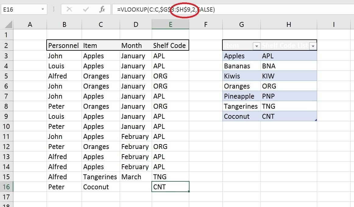
Convert the lookup table data set to a Table object.

Table object is the hero

Both advanced list solutions are dynamic thanks to the Table object. Without that object, you’d have to work much harder to make either of these advanced list solutions this flexible. To learn more about Excel Table objects, read 10 reasons to use Excel’s table object.

Send me your question about Office

I answer readers’ questions when I can, but there’s no guarantee. Don’t send files unless requested; initial requests for help that arrive with attached files will be deleted unread. You can send screenshots of your data to help clarify your question. When contacting me, be as specific as possible. For example, “Please troubleshoot my workbook and fix what’s wrong” probably won’t get a response, but “Can you tell me why this formula isn’t returning the expected results?” might. Please mention the app and version that you’re using. I’m not reimbursed by TechRepublic for my time or expertise when helping readers, nor do I ask for a fee from readers I help. You can contact me at susansalesharkins@gmail.com.

How to create two advanced dynamic lists in Excel

SEE: 30 things you should never do in Microsoft Office (free TechRepublic PDF)