


Data tells a story and while we can discover the story ourselves by reading the data, it’s quicker if the meaning is more obvious. Budgets are a good example. We don’t have time to add and subtract values in our head to learn whether or not we’ve kept actual expense items in check. We’d rather see a color or a descriptive string that clearly states whether the item is over or under budget. With Excel, you have lots of options. In this article, I’ll show you three easy ways to use budget data to share meaningful information.
More about Software
- Software Installation Policy
- Five Methods to Insert a Checkmark Into Microsoft Office Products
- How to Hide and Handle Zero Values in an Excel Chart
- How to Use Section Breaks to Control Formatting in Word
I’m using Excel 2016 on a Windows 10 64-bit system, but you can use these three solutions in older versions. For your convenience, you can download the demonstration .xls and .xlsx files. In the browser edition, you can’t add a rule using conditional formatting, but an existing format will work in the browser. In addition, you can’t apply the Subtotal feature in the browser, but the browser will display them.
SEE: How to use Excel’s what-if tools to analyze business scenarios (free PDF) (TechRepublic)
1. Expression
Adding a simple expression that subtracts the actual expenses from the budgeted expenses is a good place to start. A quick glance–is the value positive or negative–says a lot. The resulting values, shown in Figure A, tell you whether the item is over or under budget, and it tells you by how much. Enter the simple expression
=C3-D3
in cell E3 and copy it to the remaining data set.
In such a simple data set, the expression seems adequate. In a busier sheet, you might want more help.
Figure A
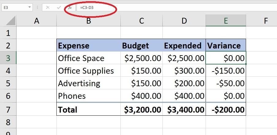
A simple expression does the trick!
2. Conditional format
Conditional formats are easy to apply, and the resulting visual impact is huge. You can use them with an ordinary range (as we’re doing) or a Table object. Our rule will build on the expression added in #1, but you can use the same logic if this column is absent–you’ll need a different expression though. Now, to add a conditional format that exposes items that are over budget, do the following:
- Select the data range–that’s B3:D6. (You could extend this to the variance and total values.)
- On the Home tab, click Conditional Formatting in the Styles group.
- From the resulting dropdown, choose New Rule.
- In the resulting dialog, click Use a formula to determine which cells to format in the upper pane.
- In the Edit the Rule Description section, enter the formula
=$E3<0 - Click the Format button and then click the Fill tab if necessary. Choose a color and click OK. Figure B shows the rule and the format.
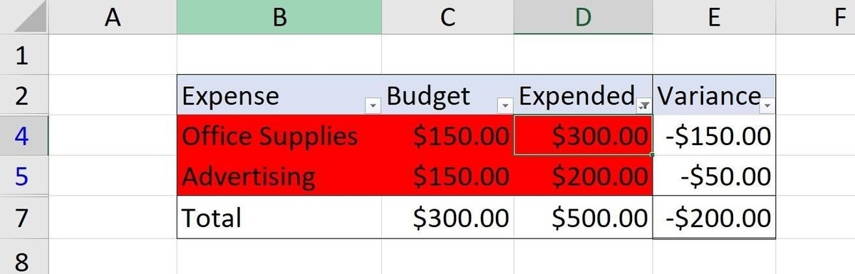
- Click OK to return the sheet. Figure C shows the new rule in place. It’s clear with a quick glance that you’ve gone over budget on office supplies and advertising.
Figure B
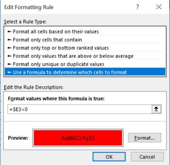
This simple rule will highlight budget items that are over budget.
Figure C
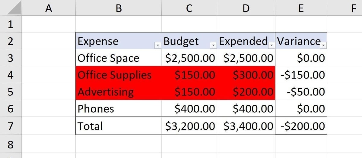
Red items are over budget.
A second rule for items under budget isn’t necessary; it’s assumed that items with no highlight are under or right on budget. However, you could add that rule using the expression =E3>=0.
Without the variance values you can achieve the same results by comparing the two budget items in their respective rules:
- =$D3>$C2 will highlight items that are over budget.
- =$D3<=$C2 will highlight items that are under or right on budget.
SEE: Windows 10 April 2018 Update: An insider’s guide (free PDF) (TechRepublic)
In-place filtering
Because the conditional format applies a fill color, you can use a filter! Click anywhere inside the data range and then click Filter on the Data tab. Click the filter dropdown for any column in the highlighted range (in this case, that excludes the Variance column). From the dropdown choose Filter By Color and then select Red (the only color in the example) as shown in Figure D. Doing so will filter out any row (budget item) that isn’t red, as you can see in Figure E. At this point, you might be done–or not.
Figure D
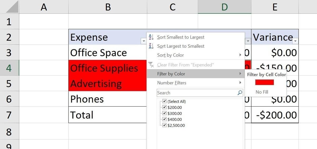
Apply a color filter.
Figure E
The filtered results.
3. Counting
Exposing over-budget items might be adequate, but let’s consider one more possibility: With the results through the end of #2, how would you count the number of items over budget? You could drop in a COUNT() function that counts values in the Variance column that are less than 0 as shown in Figure F. The functions follow:
H3: =COUNTIF(E3:E6,"<" &0)

I3: =COUNTIF(E3:E6,">=" &0)
Figure F
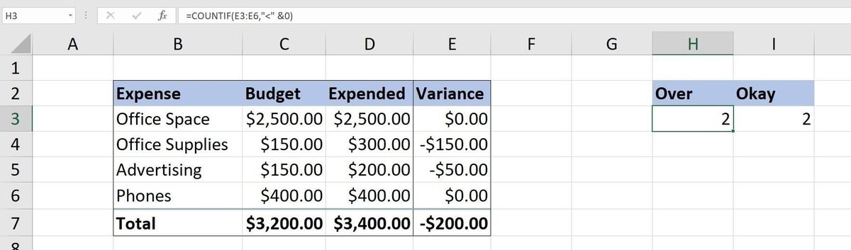
Use a simple counting expression.
A simple count might be adequate, but you might prefer to see the count within the data set itself. In this case you might consider the Subtotal feature, but there’s no common value on which to create subgroups. You’ll need a helper column to do so, so in cell F3, enter the following expression and copy it to the remaining data set, as shown in Figure G:
=IFS(E3<0,"Over",E3>=0,"Okay")
Figure G
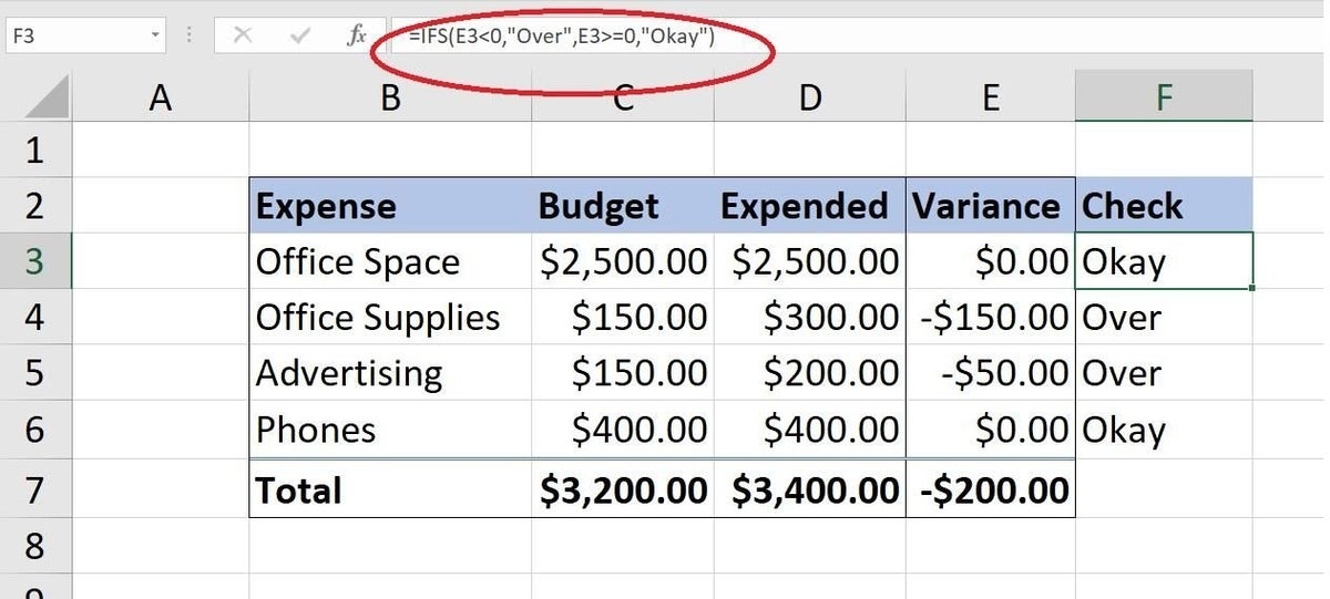
Use IFS() to return a simple count.
This simple expression returns the descriptive string values Over and Okay, accordingly. Now that you have common values, you can use Subtotal to count, as follows:
- First, sort by the Check column; Subtotal requires the sort.
- Click anywhere inside the data set.
- Click the Data tab, and then click Subtotal in the Outline group.
- In the resulting dialog, check the following settings: At each change in should be Check; Use function should be Count; Add subtotal to should be Check (Figure H).
- Click OK to see the results in Figure I.
Figure H
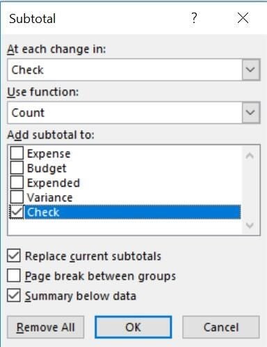
Subtotal settings.
Figure I
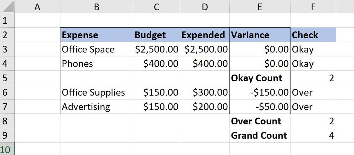
Subtotal displays counts within the data set.
In the end…
The last method is a bit convoluted, especially in a busy sheet, but is worth exploring. However, all three methods are simple and require no specialized knowledge. This example focuses on budget items, but simple expressions and formatting can be applied in almost all scenarios that need a little exposure or clarity to understand the full story.
Send me your question about Office
I answer readers’ questions when I can, but there’s no guarantee. Don’t send files unless requested; initial requests for help that arrive with attached files will be deleted unread. You can send screenshots of your data to help clarify your question. When contacting me, be as specific as possible. For example, “Please troubleshoot my workbook and fix what’s wrong” probably won’t get a response, but “Can you tell me why this formula isn’t returning the expected results?” might. Please mention the app and version that you’re using. I’m not reimbursed by TechRepublic for my time or expertise when helping readers, nor do I ask for a fee from readers I help. You can contact me at susansalesharkins@gmail.com.
Also see:
- 5 ways to delete blank rows in Excel (TechRepublic)
- How to combine and analyze data from multiple data sets using Excel Power Pivot (TechRepublic)
- How to number headings in a Word 2016 document (TechRepublic)
- Office Q&A: How to stop Excel’s paste task from overwriting destination cell’s format (TechRepublic)
- 5 ways to insert a checkmark into Office documents (TechRepublic)
- What is Microsoft 365? Microsoft’s most important subscription bundle, explained (ZDNet)