
Excel Power Pivot is a data analysis feature that’s easy to use, has a short learning curve, and most importantly is flexible and versatile enough to handle tons of data and custom needs. With a little knowledge and planning, you can turn data into meaningful information without turning to skilled database developers. It doesn’t replace database technology by any means, but it does provide a powerful tool for the user without those resources. In addition, it’s quick–you get results fast!
If you’re using Excel 2010, you must download and install Power Pivot. If you’re using Excel 2013 or 2016, it’s part of the package! I’m using Excel 2016 (desktop) on a Windows 10 64-bit system. The instructions will be similar for earlier versions. For your convenience, you can download the demonstration .xlsx file.
You might want to start by reading How to use Excel’s Data Model to turn related data into meaningful information. This article provides a basic review of the feature by walking you through the process of creating one relationship between two data sets. In this article, we’ll move forward by creating multiple relationships and adding a calculated column.
SEE: Microsoft Power BI: Getting started with data visualization (free PDF) (TechRepublic)
The data
Our example workbook has three sheets of related data: Customers, Orders, and Order Details (copied from ProductInventory.accdb, an Access database). As you can see in Figure A, the data sets are related by common fields:
- Orders.Customer and Customers.Company
- Orders.ID and Order Details.Order ID
Figure A
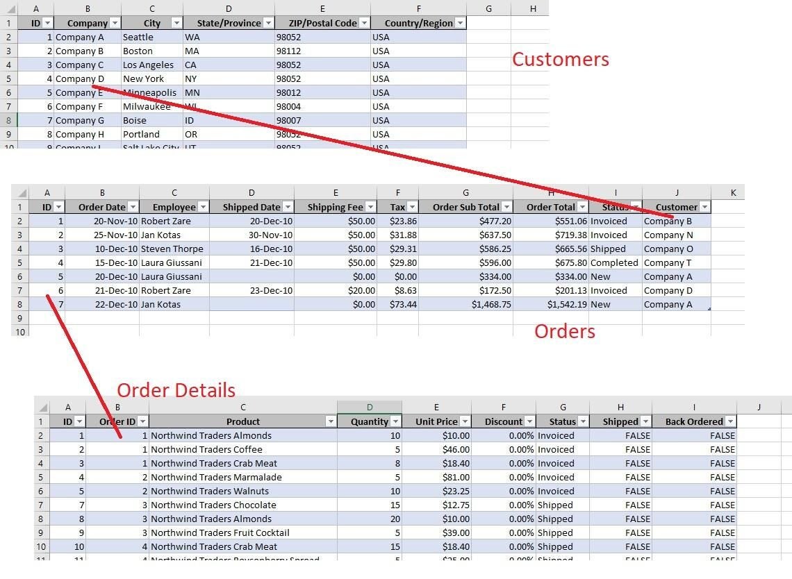
We’ll work with two relationships to combine data from three tables.
Every record in the Orders sheet represents an order. Each order in that sheet is related to a customer in the Customers sheet and details about that order in the Order Details sheet. None of the sheets alone gives the full picture. You need the data from all three sheets to pull together a complete sale.
What’s obvious at this point is that you can’t turn the data into any meaningful information–at least, not easily. For instance, viewing the Orders sheet you can see that the sub total for order 1 (before shipping and tax) is $477.20. What you don’t know is how many products compose the total or the unit price or quantity purchased for each product. Viewing the Order Details sheet, you can see all the items that compose each sale, but you don’t know who made the purchase. The Customers sheet stores information about each customer, but there’s no purchase history. That’s where Power Pivot can help. You’ll build relationships between the three data sets; with those in place, you can quickly analyze the data in meaningful ways.
As I mention in How to use Excel’s Data Model to turn related data into meaningful information, you might create complete records on a single sheet using complex formulas to lookup data. Not only is that labor intensive, the formula route consumes a lot of memory and slows things down if you have a lot of data. Fortunately, with Power Pivot, that route is unnecessary.
Convert to Table objects
Instead of connecting the sheets using formulas, we’ll use Power Pivot to create relationships between the tables. That way, you can bypass the formulas altogether. However, Power Pivot only recognizes Table objects. So, your first step is to convert each data set to a Table and name it as follows:
- Click anywhere inside the data set.
- Click the Insert tab and then click Table in the Tables group.
- In the resulting dialog, check or uncheck (as necessary) the My table has headers option. The example data sets all have headers.
- Click OK.
- Click the contextual Design tab.
- Click inside the Table Name control to the left of the ribbon and enter a meaningful name for the Table and press Enter. Naming the Table, while not necessary, will be helpful later.
Create three Table objects: Customers, OrderDetails, and Orders. When you’re done, you’re ready to continue.
SEE: Tap into the power of data validation in Excel (free PDF) (TechRepublic)
Create relationships
After converting the data sets to Table objects, you can create the relationships. To do so, click anywhere inside a Table and then click the Power Pivot tab to open the Power Pivot window. Click Add to Data Model in the Tables group. Doing so generates another view of your data. Your Excel data is safe–you can’t edit the data in the Power Pivot view. Add all three of your Table objects to Power Pivot. Figure B shows the Customers view in Power Pivot–there’s a tab for each view. (Power Pivot refers to the data sets as views.)
Figure B
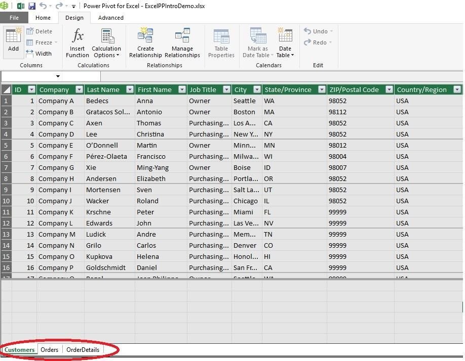
Add all three Table objects to Power Pivot.
Now let’s create the first relationship. Specifically, let’s create the relationship between Customers and Orders:
- Still in Power Pivot, click the Design tab (if necessary). Then click the Customers (view) tab (at the bottom).
- Click Create Relationship in the Relationships group. Power Pivot displays the view’s fields and a sample of the records.
- From the empty table dropdown (below), choose Orders (Figure C) and PivotTable will display its fields and records.
- Now you need to specify which field the two views share. In this case, it’s Company in the Customers Table and Customer in the Orders table. Select both fields (Figure D).
- Click OK.
Figure C
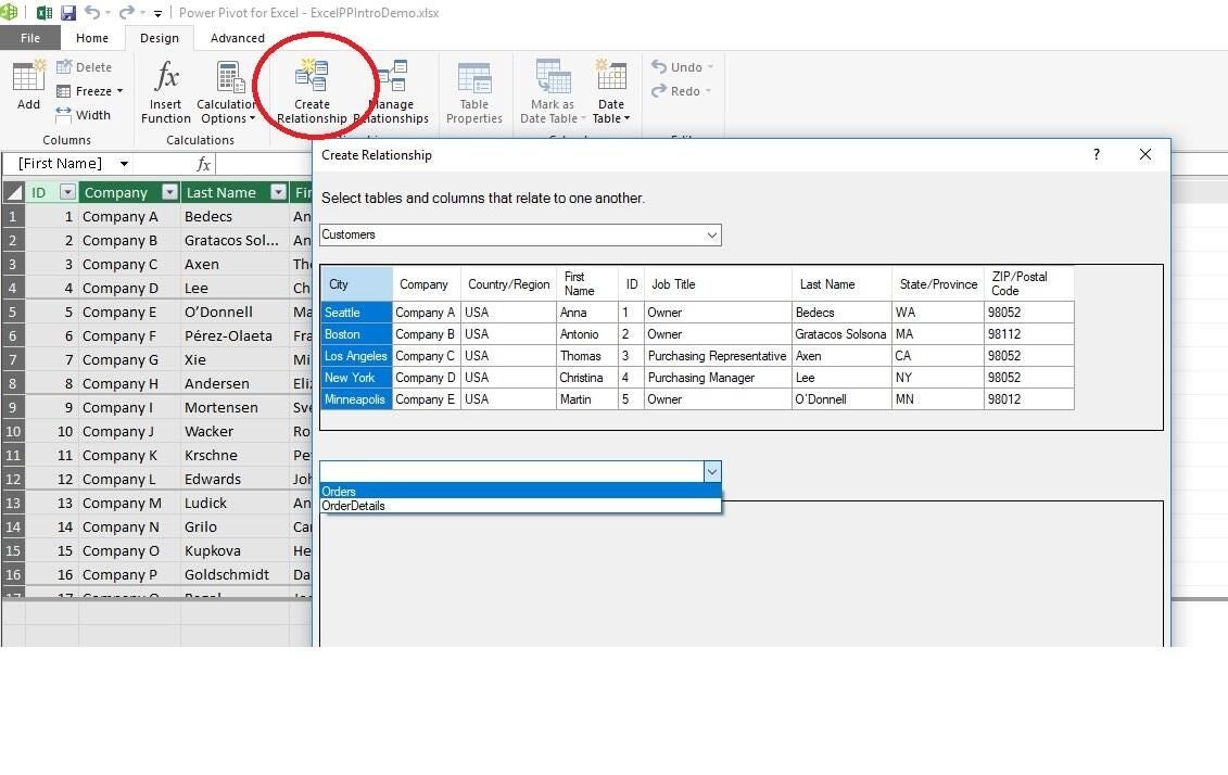
Choose a Table object.
Figure D
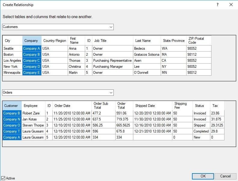
Relate the two views by a common field.
Using the instructions above and Figure E as a guide, create a relationship between Orders and OrderDetails based on the ID and Order ID fields.
Figure E
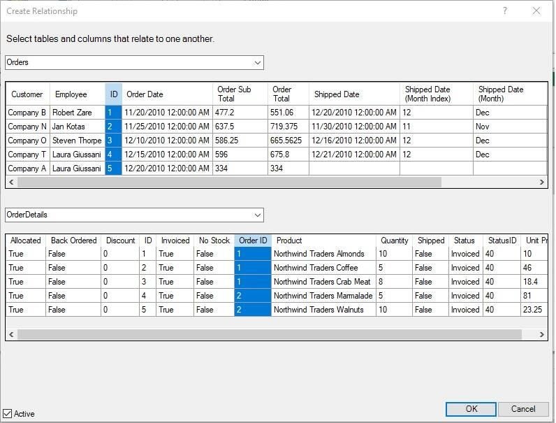
Build a relationship between Orders and OrderDetails.
At this point, we have three views based on three Table objects. There are two relationships between the three views, as you can see in Figure F. To see this yourself, click the Home tab and then click the Diagram View option in the View group.
Figure F
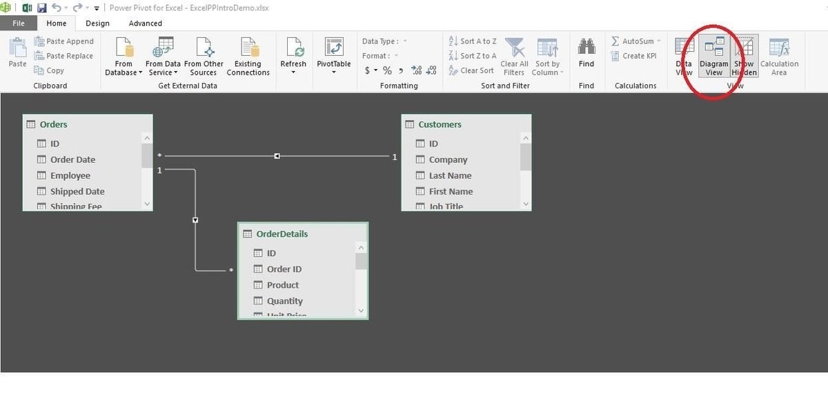
View the relationships between the views.
You now have a solid foundation on which to quickly analyze your sales data. Without formulas, you can produce meaningful information with little effort.
Build on the foundation
Now let’s put the relationships between the Power Pivot views to work. Specifically, let’s create a PivotTable that returns the costs of each item by customer and filter those results by the customers’ states and the internal personnel who made the sale.
Before we continue, let’s take a step back to review where all that data’s coming from:
- We’ll add the Company and State/Province fields from the Customers view.
- We’ll add the Product and Quantity from the OrderDetails view.
- We’ll add the Employee field from the Orders view.
Figure G shows the field list and the resulting PivotTable–the filters are in rows 1 and 2. We can filter by the state and employee, but as yet, there’s no total cost for each item.
Figure G
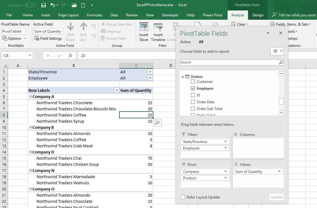
The resulting PivotTable doesn’t provide the complete results we want.
The solution is a calculated field, but you must add it to the view as follows:
- Click the Power Pivot tab and then click Manage (in the Data Model group).
- Select the OrderDetails view tab.
- Select the first cell in Add Column.
- To build the formula enter =, click the Quantity field, enter *, click the Unit Price field (Figure H), and press Enter.
- Rename the column Total (this isn’t strictly necessary but meaningful names are easier to work with).
Figure H
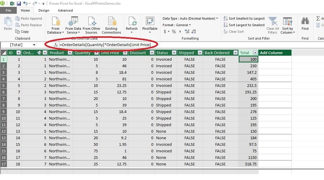
Enter the formula to return the total cost of each purchased item.
With the calculated field in place, return to the PivotTable and add the new Total field to Values. Figure I shows the results adding the Currency format to the new column.
Figure I
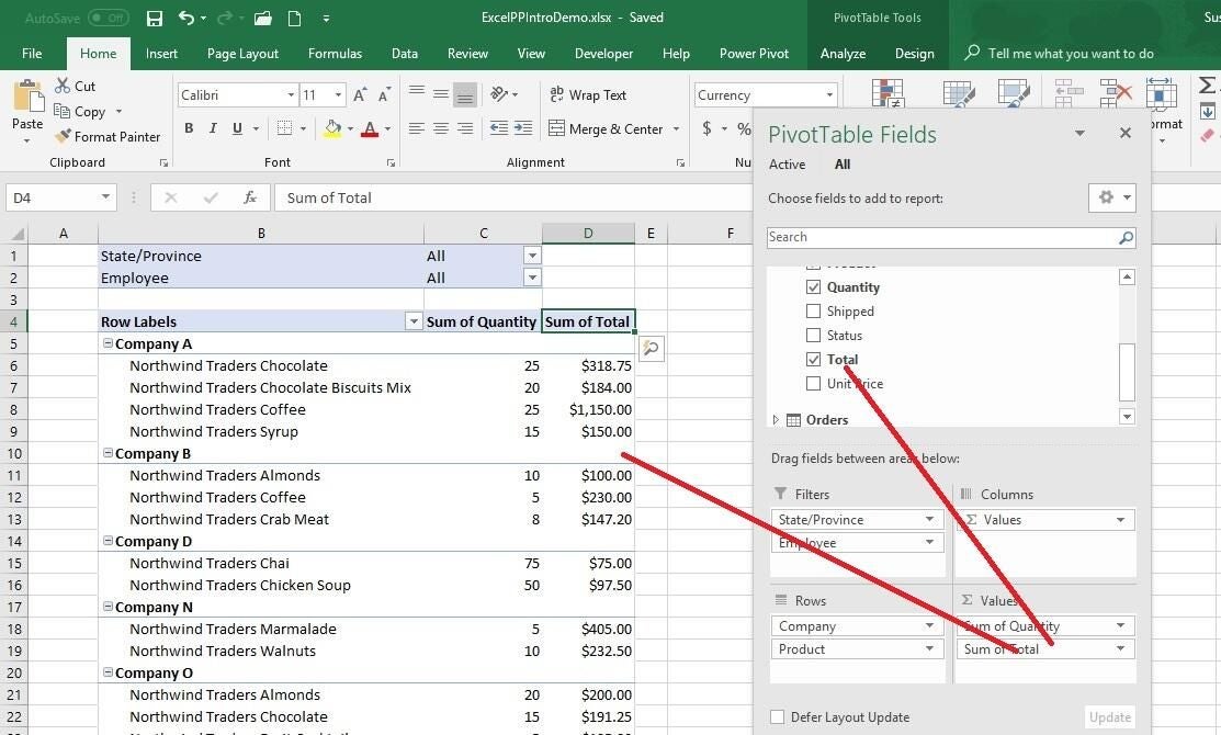
The PivotTable now displays the total sale price for individual items by company.
You can filter the results by the customers’ states and by the internal employee responsible for the sale. For instance, Figure J shows the breakdown by customers in the state of Washington–only Company A. The second filtered set shows only those Washington purchases serviced by Laura Giussani. You could easily add slicers to filter the PivotTable instead.
Figure J
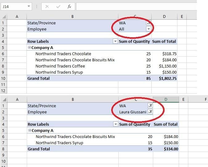
You can use the filters to focus on specific categories.
This isn’t the only way to achieve these results, but now that the relationships are in place, you can quickly pull info from all three views into meaningful information and add calculated fields to increase the value! You can think of Power Pivot as a query engine that creates a relationship between sets of related data based on a common field. That’s an over simplification, but it’s a good description.
Send me your question about Office
I answer readers’ questions when I can, but there’s no guarantee. Don’t send files unless requested; initial requests for help that arrive with attached files will be deleted unread. You can send screenshots of your data to help clarify your question. When contacting me, be as specific as possible. For example, “Please troubleshoot my workbook and fix what’s wrong” probably won’t get a response, but “Can you tell me why this formula isn’t returning the expected results?” might. Please mention the app and version that you’re using. I’m not reimbursed by TechRepublic for my time or expertise when helping readers, nor do I ask for a fee from readers I help. You can contact me at susansalesharkins@gmail.com
Also see:
- How to number headings in a Word 2016 document (TechRepublic)
- Office Q&A: How to stop Excel’s paste task from overwriting destination cell’s format (TechRepublic)
- 5 ways to insert a checkmark into Office documents (TechRepublic)
- How to control spacing and alignment in a numbered list in Microsoft Word (TechRepublic)
- How to use Excel’s Data Model to turn related data into meaningful information (TechRepublic)

