3 ways to quickly deal with blank cells in an Excel sheet

Blanks in a Microsoft Excel spreadsheet aren’t always wrong, but they can throw a monkey wrench into expressions, analyzing and reporting. I don’t recommend leaving blanks unless you have specific reason for doing so. Blanks can be troublesome and downright destructive because some functions evaluate blanks differently than values. In this article, I’ll show you three quick and easy ways to deal with blank cells:

1. using highlighting
2. entering a specific value
3. copying the value above

I’m using Microsoft 365, but you can use earlier versions. Methods two and three won’t work in Excel Online because there’s no Go To Special feature. For your convenience, you can download the .xlsx and .xls demonstration files.

SEE: 83 Excel tips every user should master (TechRepublic)

1. How to highlight blank cells in Excel

Blank cells are easy to miss if you’re working with a lot of data, so you might want to highlight them. The best way to do so is with a conditional format. As you can see in Figure A, at least one cell in each column is blank. In such a small sheet, you’d quickly see them all, but in a busy sheet with many rows and columns, blanks are easy to miss unless you do something to make them stand out, which is what we’ll do now:

1. Select the data range with blanks; in this case, that’s B3:E13. (You could select a single column.)
2. On the Home tab, click the Conditional Formatting dropdown in the Styles group.
3. Choose Highlight Cell Rules and then choose More Rules from the resulting dropdown. (In Excel Online, choose New Rule.)
4. Change the Cell Value setting in the Format Only Cells With dropdown to Blanks (Figure A).
5. Click the Format button.
6. In the resulting dialog, click the Fill tab and choose yellow for the fill color and click OK twice to see the results in Figure B.

Figure A

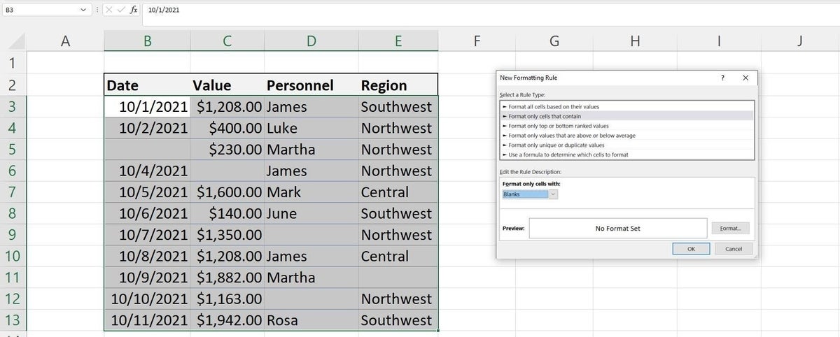
Figure B

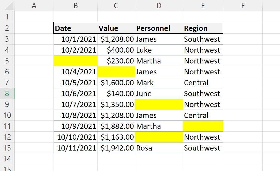
While this visual clue is helpful, you might not want blank cells at all. That means filling them with some kind of value.

2. How to fill with a specific value in Excel

Sometimes you’ll want to fill blanks with a specific value. For instance, the Accounting format enters a dash when you enter a 0, but that’s not exactly the same thing as filling a blank with a specific value. When this is the case, use the Go To dialog as follows:

1. Select the data set B3:E13.
2. Press [F5] to display the Go To dialog.
3. Click Special (in the bottom-left corner).
4. Click Blanks in the resulting dialog shown in Figure C and click OK. Doing so will select only the blank cells in the selected range.
5. Don’t click anywhere else at this point. Instead, enter a dash ( – ) as the fill value.
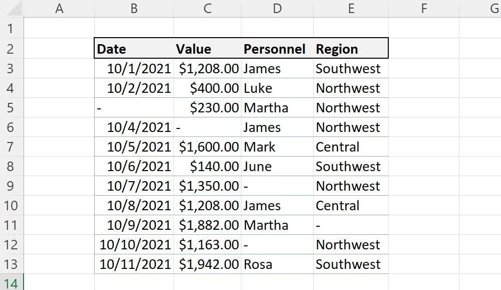
6. Instead of pressing Enter, press Ctrl + Enter to enter the dash symbol in all of the selected blank cells, as shown in Figure D.

Figure C

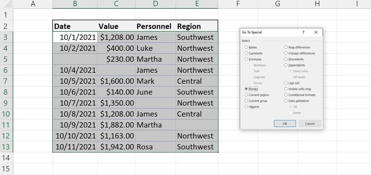
Figure D

This isn’t a dynamic solution. As you update data and add more blanks, you’ll need to run this quick task again. In this example, you entered a specific value, but that won’t always be what you want. In the next section, we’ll use same method to repeat the value above the blank cell.

3. Repeat the value above in Excel

Depending on where you receive your data, you might find that some blank cells should contain the value in the cell above. When this happens, you’ll probably want to fill in those blanks right away. If you have only a few, use the fill handle. If you have several, the fill handle is too time consuming. We’ll continue to work with the same data, even thought it’s a bit contrived within this context. Specifically, we’ll use the Go To feature to fill the missing values, but this time, we’ll enter a formula instead of a specific value:

1. Select B3:E13.
2. Press [F5] to display the Go To dialog.
3. Click Special.
4. Click Blanks in the resulting dialog and click OK.
5. Don’t click anywhere else at this point. Instead, enter a simple expression that references the cell above the blank anchor cell, or active cell. In this case, that’s B5, so enter =B4 (Figure E).
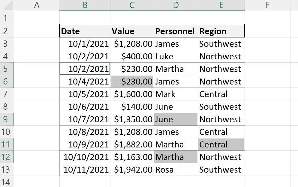
6. Press Ctrl + Enter to enter the relative reference in each of the blank cells, as shown in Figure F.

Figure E

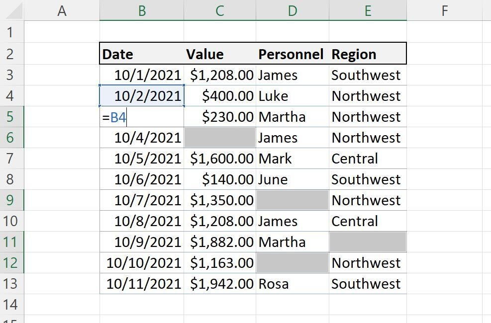
Figure F

At this point, you have a mixture of literal values and expressions. If you sort, those expressions won’t repeat the right data. You might think that won’t ever happen, but I do recommend that you change those expressions to literal values, just in case. It’s easy to forget that you’re working with a mixture of literals and expressions, and you might end up with erroneous data. Fortunately, this task is quick and easy:

1. Select B3:E13.
2. Click Copy in the Clipboard group (on the Home tab).
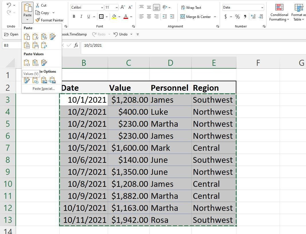
3. Next, click Paste and choose Values in the Paste Values section shown in Figure G. Doing so will replace each of the expressions with the returned value.

Figure G

These three techniques aren’t interchangeable; the way you’re using your data will determine which method you choose.