4 tips for refreshing Excel PivotTable objects

PivotTable objects are only as good as their underlying data and that can change quickly. If the pivot tables are part of a dashboard, they might not reflect updates at the source level. Depending on the information your pivot tables convey, refreshing might be extremely important, so in this article, I’ll share four tips that should help make the refresh process easy and flexible.

I’m using Office 365’s Excel 2016 (desktop), but these tips apply to earlier versions. You can refresh single pivot tables in the browser, but the Analyze contextual tab isn’t accessible; nor can you set PivotTable options. There’s no demonstration file; you won’t need one.

SEE: Software Usage Policy (Tech Pro Research)

How to refresh

Before we look at refreshing tips, let’s quickly review how to refresh pivot tables. To refresh only the current pivot table, right-click it and choose Refresh from the resulting submenu. Or, choose Refresh from the Refresh dropdown in the Data group (on the contextual Analyze tab). You can also press Alt+F5.

There are two quick ways to refresh all pivot tables in the current workbook at the same time. First, click inside any pivot table to access the contextual Analyze tab. Then, choose Refresh All from the Refresh option in the Data group. Second, press Ctrl+Alt+F5.

1. Refresh when opening the workbook

Users won’t always remember to refresh after changing the underlying data. In addition, if the pivot tables are linked to an external source, you’ll certainly want current values. The best way to guarantee that viewers see the most up-to-date information is to force Excel to update pivot tables when you open the file, as follows:

1. Right-click any pivot table and choose PivotTable Options from the resulting submenu.
2. In the resulting dialog, click the Data tab.
3. Check the Refresh data when opening the file option (Figure A).
4. Click OK and confirm the change.

Figure A

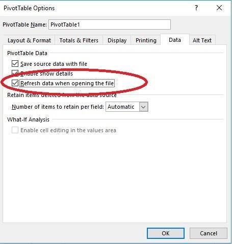
Checking this option will update the selected pivot table or all pivot tables with the same data source. If you have other pivot tables, be sure to set this option for all that have a different data source.

2. Refresh at intervals

Depending on how critical data is or if the pivot table is part of a dashboard, you might need to refresh often, which is annoying. Excel can update the pivot table at intervals to ensure viewers get the current data. You’ll have to save the pivot table to the data model when you create it as follows:

1. Click anywhere inside the data set.
2. Click the Insert tab, and then click PivotTable in the Tables group.
3. In the resulting dialog, check the Add this data to the Data Model option (Figure B).
4. Change any other settings.
5. Click OK. (Adding data to the data model can take a minute.)

Figure B

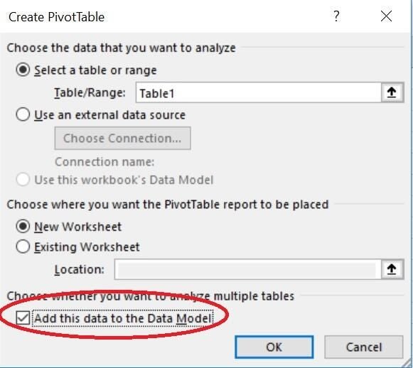
At this point, arrange the pivot table as you normally would. When you’re done, you can set the interval as follows:

1. Click anywhere inside the pivot table.
2. Click the contextual Analyze tab, and then choose Connection Properties from the Change Data Source dropdown (in the Data group).
3. In the resulting dialog, check the Refresh every option in the Refresh control section. To the right, enter an interval in minutes (Figure C).
4. Click OK.

Figure C

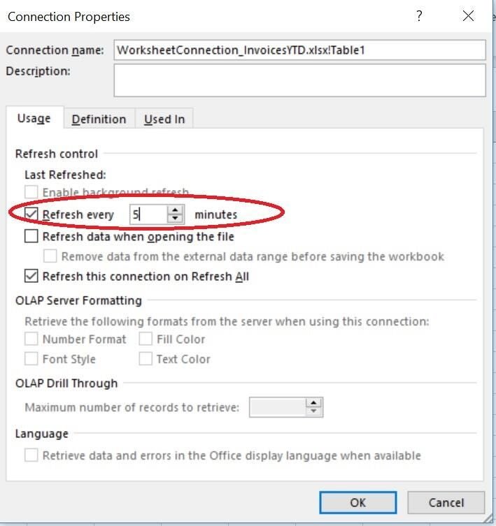
This setting is particularly helpful for dashboards and external data sources.

3. Preserve cell formatting

It’s irritating to add direct formatting to a finished pivot table, only to have it disappear when you refresh the pivot table. Perhaps you bold a few headings or add a fill color to highlight a particularly important value. Why spend your time if Excel’s going to remove it? Fortunately, you can tell Excel to keep its hands off your direct formatting as follows:

1. Right-click the pivot table and choose PivotTable Options from the resulting submenu.
2. Click the Layout & Format tab.
3. At the bottom of the options, check Preserve cell formatting on update (Figure D).
4. Click OK.

Figure D

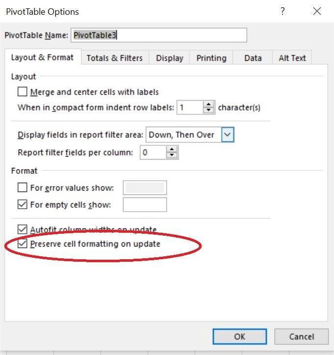
It’s an easy way to save yourself a lot of frustration.

4. Disable AutoFit

Pivot tables use an autofit column width by default. As you arrange your data, you might increase the width of columns, only to have them snap back to autofit when you refresh the pivot table. Similar to preserving direct formatting, you can disable the autofit default as follows:

1. Right-click anywhere inside the pivot table.
2. Click the Layout & Format tab.
3. Uncheck the Autofit column widths on update option (Figure E).
4. Click OK.

Figure E

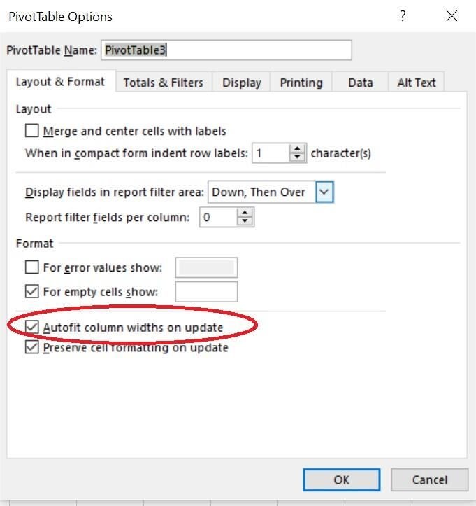
After disabling this feature, custom column widths will persist after refreshing.

Send me your question about Office

I answer readers’ questions when I can, but there’s no guarantee. Don’t send files unless requested; initial requests for help that arrive with attached files will be deleted unread. You can send screenshots of your data to help clarify your question. When contacting me, be as specific as possible. For example, “Please troubleshoot my workbook and fix what’s wrong” probably won’t get a response, but “Can you tell me why this formula isn’t returning the expected results?” might. Please mention the app and version that you’re using. I’m not reimbursed by TechRepublic for my time or expertise when helping readers, nor do I ask for a fee from readers I help. You can contact me at susansalesharkins@gmail.com.

See also

• Office Q&A: Excel referencing, Word field codes, and a table trick (TechRepublic)
• 2 ways to annotate a Word table of contents (TechRepublic)
• Use Excel data validation to prevent duplicate values in a column (TechRepublic)
• A super easy way to generate new records from multi-value columns using Excel Power Query (TechRepublic)
• 3 ways to add glossary terms to a Microsoft Word 2016 document (TechRepublic)
• Excel errors: How Microsoft’s spreadsheet may be hazardous to your health (ZDNet)
• Microsoft to add new geography, stocks data types to Excel (ZDNet)