How to display the top n records in an Excel PivotTable using built-in options

In a previous TechRepublic article, How to highlight the top n values in a Microsoft Excel sheet, I explain two different conditional formatting methods to highlight the top n values in a data set in Microsoft Excel. Either is reasonable when you want to view all of the data. When you want to see only the top n records—filtering out all other records—you’ll need a different strategy.

Disclosure: TechRepublic may earn a commission from some of the products featured on this page. TechRepublic and the author were not compensated for this independent review.

Fortunately, Microsoft Excel has a built-in filter for PivotTables that will let you display the top (or bottom) n record. In this article, you’ll create a simple PivotTable and then use the built-in filter to display only the top 10 records in the data source. Then, we’ll discuss some problems with the results and possible solutions. It’s this latter section of the article that might provide the most new material for some of you.

I’m using (desktop) Office 365, but you can use earlier versions of the ribbon format. You can work with your own data or download the demonstration .xlsx file (this article isn’t applicable to the older .xls version). The browser edition will display the PivotTable, but you can’t run code in the browser.

How to build a PivotTable in Excel

This section is a tutorial on building a PivotTable. If you know how to build one, you can skip this section. To build the demonstration PivotTable using the data set in Figure A, do the following:

1. Click anywhere inside the data set and then click the Insert tab. In the Tables group, click PivotTable.
2. In the resulting dialog, click OK; we don’t need to change any default settings.
3. Click inside the PivotTable frame. In the PivotTable field list pane, drag Product Name to the Rows section. Drag Unit Price to the Values section (Figure B). The frame will update accordingly as you add fields.

Figure A

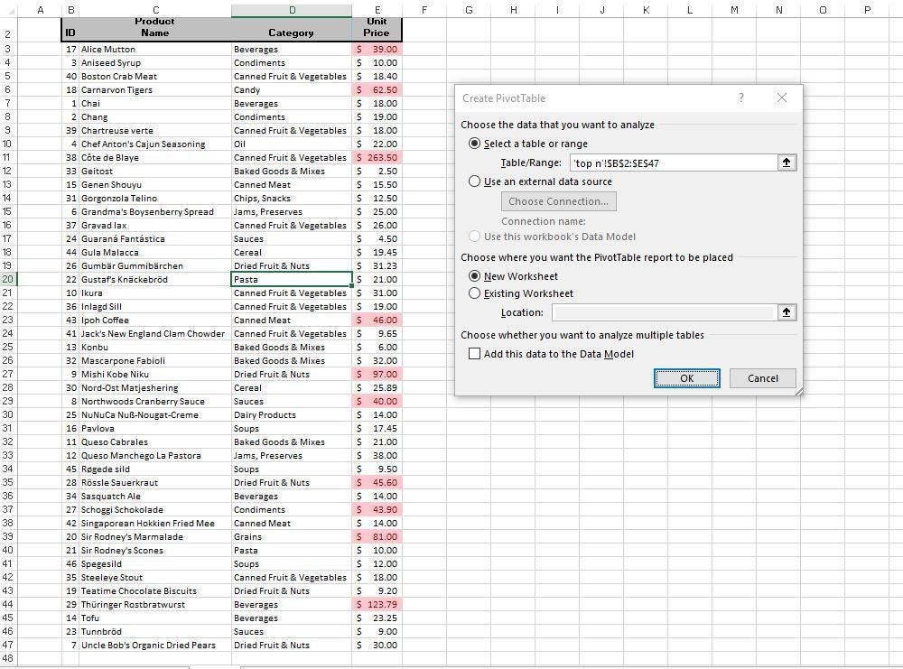
Figure B

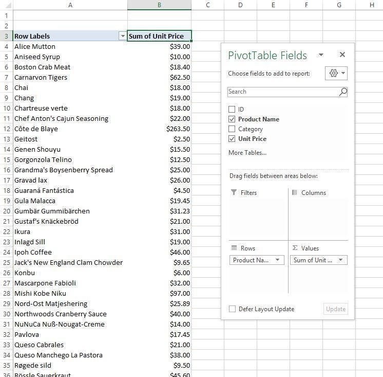
By default, the PivotTable sums the unit price values by products, but our list of products is unique, so none of the values change. To format the unit price column, right-click the header cell and choose Number Format from the resulting submenu. (I chose Currency.)

As is, the PivotTable displays all the records. Let’s look at our first method for displaying the top n unit price values.

How to use the built-in option

Applying a filter is easy, and there are lots of options. The downside is they’re not dynamic, but we’ll discuss that in a bit. Now, let’s apply that filter:

1. Click the Row Labels dropdown filter.
2. Choose Value Filters (remember, we’re evaluating the unit price values, not the products), and then choose Top 10 (Figure C). There’s no dropdown for the unit price column because it’s a values column. There are lots of options, so you’ll want to explore those later.
3. The resulting dialog has several options, but the default settings (Figure D) are perfect for our example: display the top 10 items in the Sum of Unit Price column.
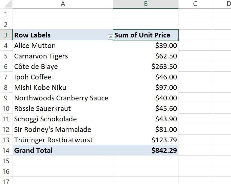
4. Click OK to see the results in Figure E.

Figure C

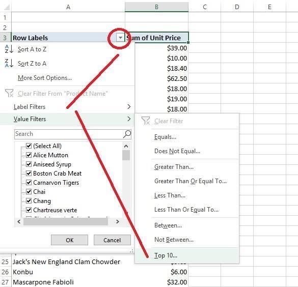
Figure D

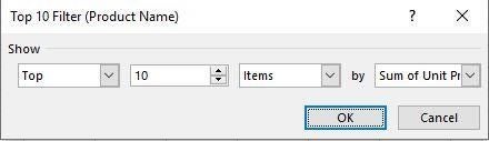
Figure E

You could use the resulting PivotTable as is, but there are a few issues you might want to consider first. Let’s take a look next.

Fixing a few small problems

Now, let’s tweak the results a bit. In this case, the totaling row at the bottom isn’t meaningful, so you can turn it off. To do so, click the contextual Design tab. In the Layout group, click the Grand Totals dropdown and choose Off for Rows and Columns.

Excel sorts by the row label—products—so it can group and sum multiple values correctly. In this case, it’s unnecessary and the product sort isn’t particularly meaningful. Most likely, you’ll want to sort by the unit price. To do so, right-click any unit price cell, choose Sort, and then choose Sort Largest to Smallest. The header text isn’t descriptive. To change it, simply click inside the cell and replace the default headers–or not. If you decide to hide the dropdown arrow, you can skip this step.

Most likely, you’ll not want viewers to change the filter. There are a few complex methods for doing so, but the easiest is to remove the filter dropdown. To do so, click anywhere inside the PivotTable and click the contextual PivotTable Analyze tab. Then, click the Options dropdown in the PivotTable group (to the far left), and choose Options. In the resulting dialog, click the Display tab and uncheck the Display field caption and filter drop downs option. Doing so will inhibit both the header text and the dropdown, which isn’t really a problem. Simply hide the row and add the appropriate text or title above the PivotTable. (This option isn’t used in the demonstration file.)

If you’re not familiar with PivotTables, here’s an important behavior that you need to remember: They don’t update automatically. If you change a value in the source data that would impact the top 10 PivotTable, the PivotTable will not display that change until you refresh it. But there is help, if not a perfect solution.

A not-so-dynamic workaround

To update a PivotTable, right-click any cell and choose Refresh. Viewers won’t know to do this though, so the display can be behind updates. The simplest solution is to force Excel to update PivotTables when someone opens the workbook. You can do so, as follows:

1. Click anywhere inside the PivotTable and then click the contextual PivotTable Analyze tab.
2. In the PivotTable group (to the far left), click the Options dropdown (under the PivotTable Name box), and choose Options from the dropdown list.
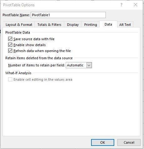
3. In the resulting dialog, click the Data tab.
4. Check the Refresh data when opening the file option (Figure F).
5. Click OK.

Figure F

Choosing this option assures that viewers see the most up-to-date information, but they have to open the file, so it’s not a perfect fix for the problem. (This option isn’t set in the demonstration file so you can experience the behavior for yourself.) Perhaps a better solution is the simple event procedure in Listing A.

Listing A

Private Sub Worksheet_Deactivate()

ThisWorkbook.RefreshAll

End Sub

Add this procedure to the sheet module attached to the data source. When you update the data and then leave that sheet, the Deactivate method triggers a refresh method. This easy solution comes with a few limitations. First, the PivotTable and the data source must be on different sheets. In addition, the RefreshAll method refreshes everything: all PivotTables, queries, and so on. If you want to limit the refresh to the PivotTable, use the following refresh method instead:

sheetname.PivotTables(“pivottablename“).PivotCache.Refresh

Be sure to update sheetname and pivottablename accordingly when applying to your own work. The demonstration file contains the code, but it’s commented out. When applying code to your own work, don’t copy from this web page because the Visual Basic Editor (VBE) will be unable to compile unseen characters. Enter the code yourself or copy the code into Word (or another text editor) and then copy the code from there into the VBE. In addition, if you add the code to your workbook, be sure to save the file as a macro-enabled workbook (.xlsm).

Send me your Microsoft Office questions

I answer readers’ questions when I can, but there’s no guarantee. Don’t send files unless requested; initial requests for help that arrive with attached files will be deleted unread. You can send screenshots of your data to help clarify your question. When contacting me, be as specific as possible. For example, “Please troubleshoot my workbook and fix what’s wrong” probably won’t get a response, but “Can you tell me why this formula isn’t returning the expected results?” might. Please mention the app and version that you’re using. I’m not reimbursed by TechRepublic for my time or expertise when helping readers, nor do I ask for a fee from readers I help. You can contact me at susansalesharkins@gmail.com.