


Image: filmfoto, Getty Images/iStockphoto
Must-read Windows coverage
- CrowdStrike Outage Disrupts Microsoft Systems Worldwide
- 10 Best Project Management Software for Windows in 2024
- Windows 10 Extended Security Updates Promised for Small Businesses and Home Users
- Securing Windows Policy
Dashboard views are usually flexible, allowing the viewer to change criteria easily. For instance, a viewer might want to see the top 10 values in a data set. Other viewers might want to see only the top value, or the top five, or the top three, and so on. Fortunately, Microsoft Excel’s conditional formatting feature can do this without much work. In this article, I’ll show you two conditional formats that highlight the top values in a data set: One isn’t flexible enough for a dashboard setting but another is.
Disclosure: TechRepublic may earn a commission from some of the products featured on this page. TechRepublic and the author were not compensated for this independent review.
I’m using (desktop) Office 365 on a Windows 10 64-bit system, but this will work in earlier versions. You can work with the downloadable .xlsx file. This solution isn’t supported by the earlier menu versions. The browser edition will support the .xlsx conditional formats in an existing file. You can apply the built-in top rule online, but you can’t apply the formulaic rule online.
How to use the built-in rule in Microsoft Excel
Excel offers a few built-in conditional rules for formatting top and bottom values. They’re easy to use, but they’re not dynamic. You can change n, but you must do so through the interface. That means viewers can’t change the number on the fly.
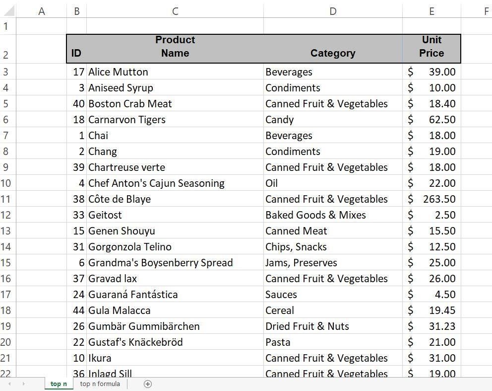
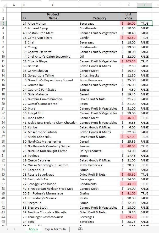
Let’s take a look at the rule anyway because it’s easy to implement and works well when you don’t need more flexibility. Using the simple data set (partially) shown in Figure A, we’ll use a built-in conditional rule to highlight the top 10 product prices.
Figure A
Now, let’s highlight the top 10 product prices as follows:
- Select the product prices, E3:E47. It’s not necessary to sort first. In addition, if you want to highlight the entire rows, select B3:E47.
- In the Styles group (Home tab), click Conditional Formatting and choose Top/Bottom Rules from the dropdown (Figure B).
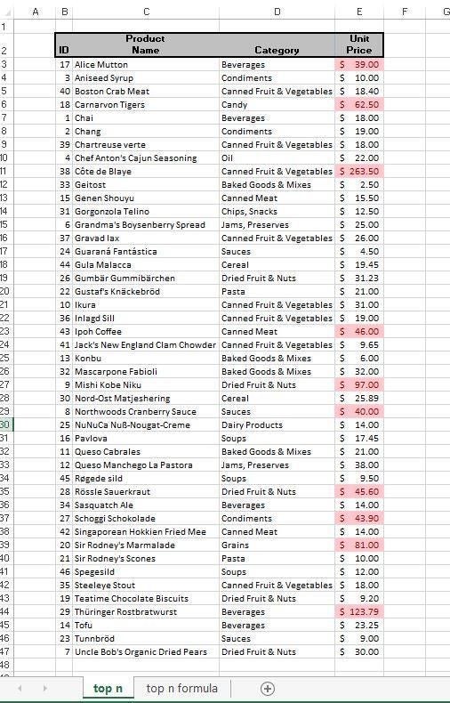
- The dropdown to the left lets you control n—you can choose any value, but the default is 10 (Figure C). Use the dropdown to the right to choose from a number of fixed formats. Figure D shows the results of retaining both default settings.
Figure B
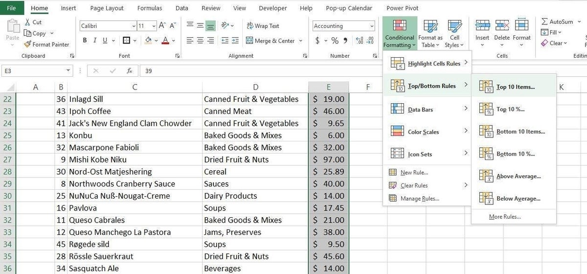
Figure C
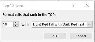
Figure D
You can set n to any value while creating the rule, but you can’t change it on the fly. To do so, you’ll need a formulaic rule.
SEE: How to use color in a PowerPoint slide to highlight information (TechRepublic)
How to use a formula
If you want a more flexible review of the top n records, you’ll need a formula. To that end, you’ll add an input cell for the user to identify n. The conditional format rule will reference the input cell to determine how many of the top values to format. You could limit the number or limit the data type by using a validation control, but we’re going to skip that step. It’s something to consider when applying this to your own work, though.
The formula uses the form:
anchor>=LARGE(range,n)
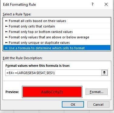
Excel’s LARGE() function returns the nth largest value in range. Using our form, we can expand n to be inclusive. For our demonstration sheet, the following formula:
E4>=LARGE($E$4:$E$47,10)
returns TRUE when the current value is within the results of LARGE(). Figure E shows this formula next to the highlighted values from the previous example. Instead of using the value 10 in the formula, we’ll reference the input cell E1:
E4>=LARGE($E$4:$E$47,$E$1)
The TRUE/FALSE formula in column F isn’t necessary; it’s a visual aid.
Figure E
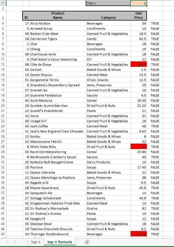
Before adding the new rule, insert a few rows above the data set to accommodate the input cell (Figure G). Now, let’s use the formula as follows:
- Select E4:E48. (The cell reference includes the newly inserted rows, so it isn’t the same as the first example’s.)
- In the Styles group, click Conditional Formatting and choose New Rule from the dropdown.
- Select the last rule in the top pane.
- In the resulting control below, enter the formula
E4>=LARGE($E$4:$E$47,$E$1) - Click the Format tab.
- Click the Fill tab, choose a color, and click OK. Figure F shows the formula and the format.
- Click OK again to return to the sheet, which appears to do nothing at this point. That’s because there’s no value in the input cell.
Figure F
SEE: How to use Outlook’s Quick Step feature to save time sending email (TechRepublic)
Enter a value, such as 3, in the input cell E1 to see the results shown in Figure G. As you can see, the rule highlights the top three values. Change the input value to 5, to 7, and so on. Because this solution is dynamic, it’s a great one to use in a dashboard setting. The formula rule works equally as well with a Table object and will even update as you delete and add new records.
Figure G
Send me your Microsoft Office questions
I answer readers’ questions when I can, but there’s no guarantee. Don’t send files unless requested; initial requests for help that arrive with attached files will be deleted unread. You can send screenshots of your data to help clarify your question. When contacting me, be as specific as possible. For example, “Please troubleshoot my workbook and fix what’s wrong” probably won’t get a response, but “Can you tell me why this formula isn’t returning the expected results?” might. Please mention the app and version that you’re using. I’m not reimbursed by TechRepublic for my time or expertise when helping readers, nor do I ask for a fee from readers I help. You can contact me at susansalesharkins@gmail.com.