How to use conditional formatting to compare values from row to row, or not, in Excel

Conditional formatting in Microsoft Excel has been around for a long time, but I find that most rules evaluate columns; it’s rarely that simple, but it’s fair to say that most conditional rules compare values from one column to another. It’s inherent to the way we structure data. However, occasionally we need to compare values from one row to another. The good news is that it’s no more difficult to implement a row-comparing formatting rule than to compare columns. In this article, we’ll use a rule to compare values from row to row. But the crux is, anytime you’re comparing one value to another, whether by columns or rows, you might not get the results you expect.

SEE: 83 Excel tips every user should master (TechRepublic)

I’m using Microsoft 365 on a Windows 10 64-bit system. (Try to hold off upgrading to Windows 11 until all the kinks are worked out.) Excel Online will display existing conditional formats and allow you to add built-in rules. You can’t, however, apply expressions as rules. For your convenience, you can download the demonstration .xlsx and .xls files.

The format requirement

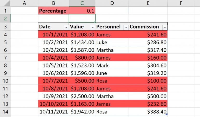
Let’s keep this as simple as possible for now. Let’s suppose that you want to know when a commission seems a bit lower than usual. Figure A shows a simple tracking sheet for sales and commissions for five employees using a Table object, although, you can do the same using a normal data range. Let’s suppose you want to know if a percentage is lower than expected, when compared with the commission in the row above. Now, this won’t really give us the analysis we’d truly need in this situation, but it does give us a bit of a contrived example for comparing values from row to row. We’ll deal with the logical flaw later.

Figure A

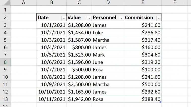
To accomplish this simple requirement, let’s highlight commission amounts that are 25% lower than the row above:

1. Select the data set—in this case, B4:E14. If you want to highlight only the commission cell, select only that column of values. But for this example, I want to highlight the entire record.
2. Click the Home tab, click Conditional Formatting in the Styles group, and then choose New Rule from the dropdown list.
3. In the top pane, select Use a Formula to Determine Which Cells to Format.
4. In the bottom pane, enter the expression =$E4<($E5 - ($E5 *0.25)). That period following the )) characters is punctuation, and not part of the expression.
5. Click the Format button, click the Fill tab, and then choose a highlight color. I choose red because we’re looking for lower values.
6. Click OK to return to the first pane, which shows the rule and the format (Figure B).
7. Click OK to apply the format and return to the sheet, shown in Figure C. For now, don’t worry about the cells in row 1. We’ll use them in a bit.

Figure B

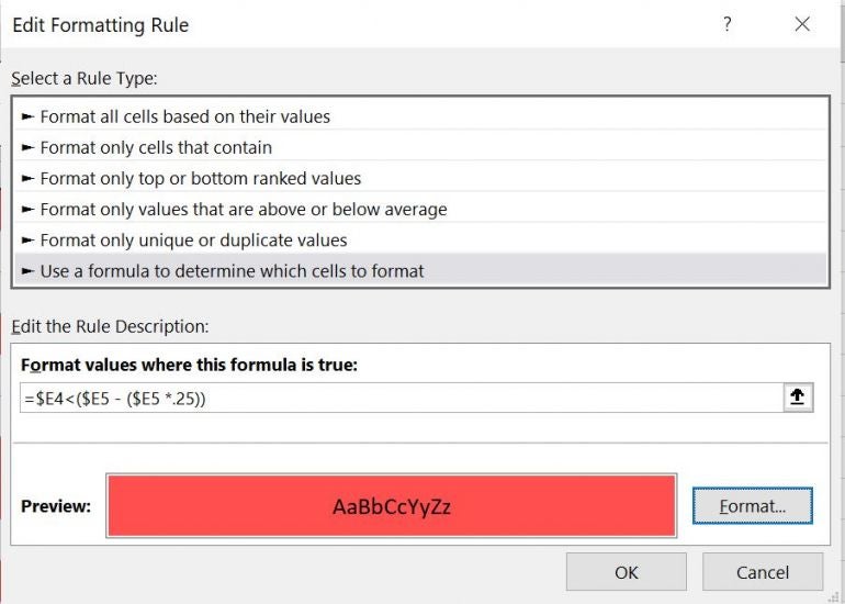
Figure C

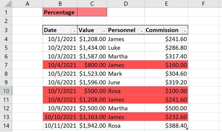
With a quick review, all seems well, except for the value in E11. When compared with the other commissions, it seems right in line. The problem is the value it’s compared with: $500 in E12. The rule is working as it should. Remember, we’re not comparing the entire set of commission values as a whole. We’re comparing them from one row to another. Yes, it doesn’t work as well as we might like because it’s a bit contrived, on purpose, so you can see how easy it is to think you’ve got the logic correct, only to find a flaw.

It’s important to note that the absolute referencing for column E is essential if you want to format the entire cell. Similarly, the row must be relative.

At this point, you might be wondering about the formatted cells in row 1. C1 is an input cell. By referencing the percentage this way, you can change the percentage on the fly without modifying the actual rule.

How to modify the rule

By adding an input cell, you can quickly update the percentage used in the conditional rule. Let’s do that now:

1. Click the Home tab, click Conditional Formatting in the Styles group, and then choose Manage Rules from the dropdown list.
2. From the Show Formatting Rules dropdown, choose This Worksheet.
3. In the resulting pane, select the rule and choose Edit Rule in the menu row above.
4. Click inside the rule and press F2 so you can edit it easily.
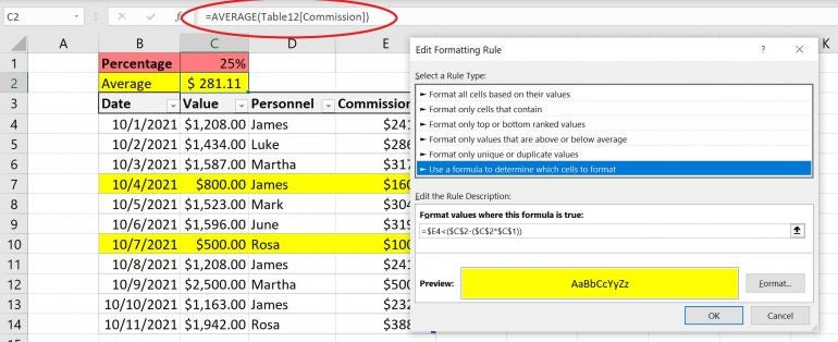
5. Replace the 0.25 value with an absolute reference to $C$1 (Figure D).
6. Click OK twice to apply and return to the sheet.

Figure D

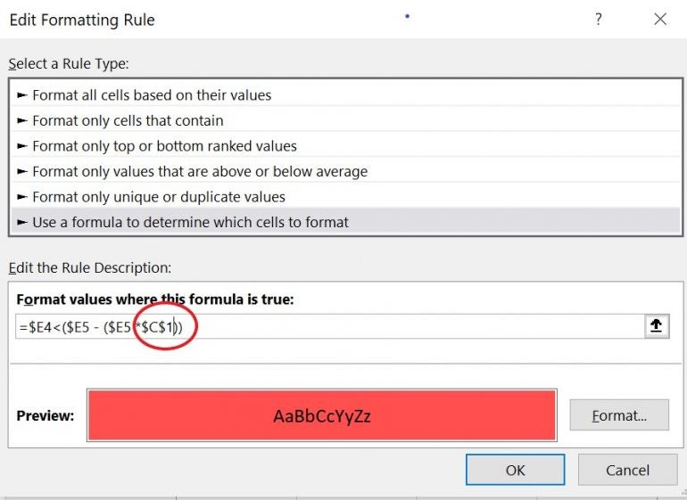
The rule won’t work correctly until you enter an input value into C1, so enter .25 now. The rule highlights the same records as before. Change .25 to .10 so you can see it update. As you can see in Figure E, the rule includes one more record, row 4. As you lower the percentage, you might increase the number of highlighted records and vice versa. If you want to highlight records that exceed the record below by a specific percentage, simply change the < sign in the rule to >. In fact, you could employ both rules, but you might choose a different color, such as green, to highlight higher than usual commissions.

Figure E

How to correct the logic

As is, the rule doesn’t work the way we might want because we’re comparing one row to another and ignoring the whole—in otherwise, the average commission. I recommend that you use the Manage Rules option to delete the current rule before you continue. It isn’t absolutely necessary, but it will be easier to see the new results.

The first thing we must consider is how to include the average commission quickly and easily in our new rule. We could add it to the rule directly, but we’ll end up with a complex rule. The easier way is to enter the averaging function in C2

=AVERAGE(Table12[Commission])

If you’re not using a Table object, enter

=AVERAGE(E4:E14)

Now, let’s fix our logic by using a new rule:

1. Select the data set and use Conditional Formatting to add a new rule, as you did earlier.
2. Enter the expression =$E4<($C$2-($C$2*$C$1)). Remember, the period isn’t included in the expression and the absolute/relative referencing is important.
3. Click the Format button, apply a fill color (I chose yellow), and click OK twice to return to the sheet.

As you can see in Figure F, this new rule highlights only two records. The new logic is more accurate to our needs. But we’ve completely eliminated the row-by-row reference in doing so, but this often happens. That’s why I started with such a contrived example. This could just as easily happen when comparing column to column.

Figure F

As before, you can change the percentage in C1 to update the entire view. In addition, if you want to see commissions that exceed the average by a specific percentage (C1), change the < in the rule to >. Finally, because we’re using a Table object, it’s all dynamic. The AVERAGE() function will update automatically as you modify, add, or delete records. If you’re using a normal data range, that won’t happen.

You might be wondering why I started with a row-by-row example only to completely eliminate it. First, I wanted a super easy example to introduce the idea of evaluating a formatting rule by rows. As I mentioned twice, referencing is critical. In addition, as with the simplest rules, sometimes they aren’t adequate, and you need to rethink your first effort. There’s nothing wrong with that; I do it all the time.