


Finding duplicate values in the same column is easy; you can sort or apply a filter depending on the circumstances. Finding duplicates that span multiple columns is a tad more difficult. A sort can work, but then you must spot the duplicates. So, while it’s better than no solution at all, it’s not a great solution. Conditional formatting might be an option, but if you already have several formats, it too might not be the best solution. If you want a solution that screams out, “Here I am! I’m a duplicate!” why not do just that? In this article, I’ll show you a simple expression solution that might be easier to implement and more effective than conditional formatting.
More about Software
- Software Installation Policy
- Five Methods to Insert a Checkmark Into Microsoft Office Products
- How to Hide and Handle Zero Values in an Excel Chart
- How to Use Section Breaks to Control Formatting in Word
I’m using Excel 2016 (desktop) on a Windows 10 system, but this solution will work in older versions. You can work with your own data or download the demonstration .xls and .xlsx files.
Note: this is the second of three articles in a series. For the previous articles, see How to use Excel’s conditional formatting to compare lists.
The example data
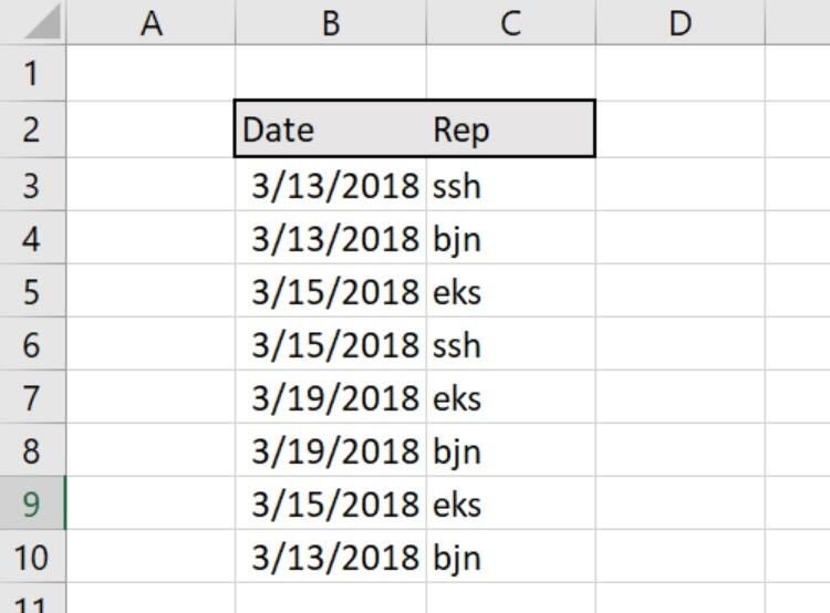
Let’s take a quick look at a simple example. The sheet shown in Figure A contains a column of dates and a column of initials. A few dates occur more than once, and a few initial sets also repeat; those represent duplicates within a single column. We’re interested in rows that repeat the same date and the same initial set. That’s what I mean by a multi-column duplicate. And, we’re assuming you don’t want to use a custom conditional rule.
Figure A
We’ll add a formula solution that spots duplicates.
It’s easy to spot the duplicates–rows 4 and 8 and rows 5 and 9–in such a simple sheet, but what if you had hundreds or thousands of rows to check? A filter works, but it’s a vulnerable solution. In this case, there are three distinct dates. That means a user must review at least three sets of records to find duplicates. Even then, you must trust your user to spot them! The built-in conditional formatting rule would highlight everything because all the values are duplicates! You might try an advanced filter or even a custom conditional format rule, but both require some hoop-jumping.
SEE: Microsoft SharePoint: A guide for business professionals (Tech Pro Research)
Concatenate
Let’s take a different approach from sort, filtering, and custom formatting. Instead, we’ll use COUNTIF() to count the number of combined values and an IF() function to return an appropriate message. The first step is to concatenate all the columns, so you’re not really comparing; you’re counting.
To concatenate the values, enter the following formula in D3 and copy it to the D4:D10:
=B3&C3
This technique is flexible, and you can concatenate several columns by combining them with the & character. Excel returns the serial values (Figure B) but that won’t interfere with the technique. (Time values might be problematic, depending on how they’re entered.)
Figure B
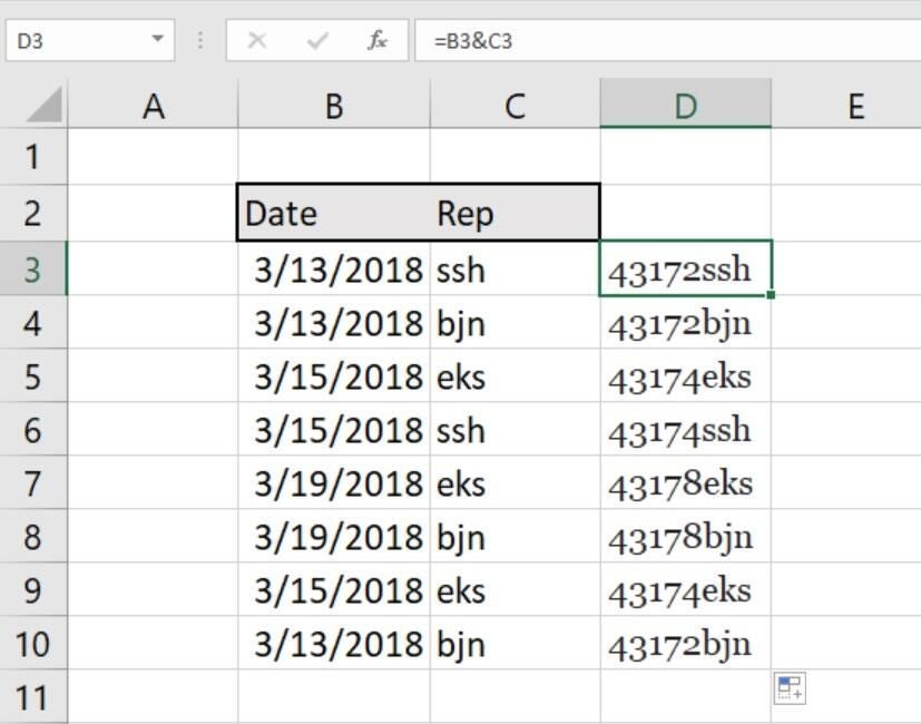
Concatenate the values.
Count
Now we’re ready to count the concatenated results in column D, so enter the formula
=IF(COUNTIF($D$3:D3,D3)>1, "Here I am! I'm a duplicate!", "Original")
in E3 and copy to the remaining cells. As you can see in Figure C, finding multi-column duplicates is as easy as sorting by column E (although this simple example doesn’t require that extra step). You could find duplicate records or subsets of records. You determine the outcome by deciding which columns to concatenate.
Figure C
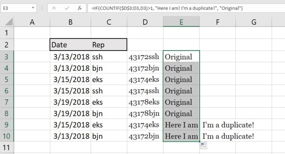
The resulting strings identify duplicate records.
The COUNTIF() function counts the number of times the concatenated result occurs within the extended range. If the count is greater than 1, the formula returns the string “Here I am! I’m a duplicate!”; otherwise, the formula returns the string “Original.” It’s important to note that the first occurrence of a duplicate evaluates as original; only duplicates following the original return the duplicate string. You could reduce the visual noise a bit by returning an empty string instead of the string, “Original” when there’s no duplicate.
This technique easily adapts to additional columns. Simply add each column to the concatenating formula. Of course, there are other ways to identify multi-column duplicates in Excel, but this one requires no specialized knowledge and is incredibly easy to implement.
SEE: Tap into the power of data validation in Excel (free PDF) (TechRepublic)
Stay tuned
In a subsequent article, we’ll continue this study of finding duplicates with a more complex example set–comparing multi-column lists in different data sets.
Send me your question about Office
I answer readers’ questions when I can, but there’s no guarantee. Don’t send files unless requested; initial requests for help that arrive with attached files will be deleted unread. You can send screenshots of your data to help clarify your question. When contacting me, be as specific as possible. For example, “Please troubleshoot my workbook and fix what’s wrong” probably won’t get a response, but “Can you tell me why this formula isn’t returning the expected results?” might. Please mention the app and version that you’re using. I’m not reimbursed by TechRepublic for my time or expertise when helping readers, nor do I ask for a fee from readers I help. You can contact me at susansalesharkins@gmail.com.
Also see:
- How to apply an Excel validation control that protects a specific limit (TechRepublic)
- Office Q&A: After-the-fact captions and easy counts using a PivotTable (TechRepublic)
- How to create transparent text in PowerPoint 2016 (TechRepublic)
- How to create a quick and easy online form with 365 Microsoft Forms (TechRepublic)
- How to build a simple timesheet in Excel 2016 (TechRepublic)
- 7 ways you can (maybe) get Microsoft Office 365 for free (ZDNet)
- You’ve been using Excel wrong all along (and that’s OK) (ZDNet)