


Comparing lists for common values, or duplicates is a task that often has many variables. You can compare values in the same list or you might want to compare one list to another. Then there’s the definition of duplicate. You’ll find many solutions if you search the internet, but you’ll find no one-size-fits-all solution. You must know your data and apply an appropriate solution.
In this article, we’ll use conditional formatting to compare lists and spot duplicates. First, we’ll apply the built-in duplicates rule to compare items in a single list; then we’ll use it to compare two lists. Next, we’ll use a custom conditional formatting rule to find duplicates when the built-in rule isn’t adequate.
More about Software
- Software Installation Policy
- Five Methods to Insert a Checkmark Into Microsoft Office Products
- How to Hide and Handle Zero Values in an Excel Chart
- How to Use Section Breaks to Control Formatting in Word
I’m using Excel 2016 (desktop) on a Windows 10 system, but these rules are available in older ribbon versions. You can work with your own data or download the demonstration .xls and .xlsx files. The browser edition supports existing conditional formatting rules and you can even apply built-in rules. You can’t however, apply custom rules in the browser.
Built-in rule
You can use a formula with conditional formatting to compare data, but sometimes the built-in rules can get the job done. You’ll need no specialized knowledge, but you should understand how the feature works to avoid frustration. To illustrate, we’ll first look at how the built-in rule compares items in a single list, using the simple sheet shown in Figure A as follows:
- Select the first list, B1:B12. (I repeated the last item on purpose.)
- On the Home tab, click Conditional Formatting in the Styles group.
- Choose Highlight Cells Rules and then select Duplicates Values in the subsequent menu (Figure A).
- In the resulting dialog, select an appropriate format and click OK. As you can in Figure B, this built-in rule highlighted duplicates in the same column because we selected a single column.
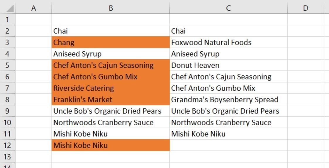
Figure A
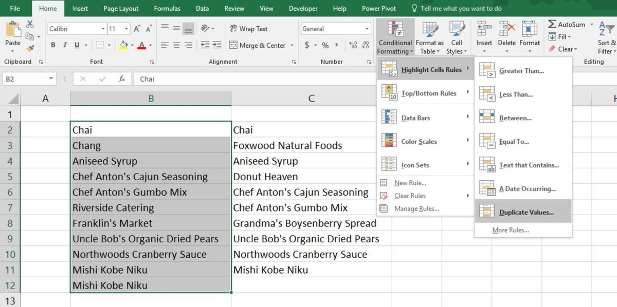
This built-in duplicate rule compares items in a single list.
Figure B
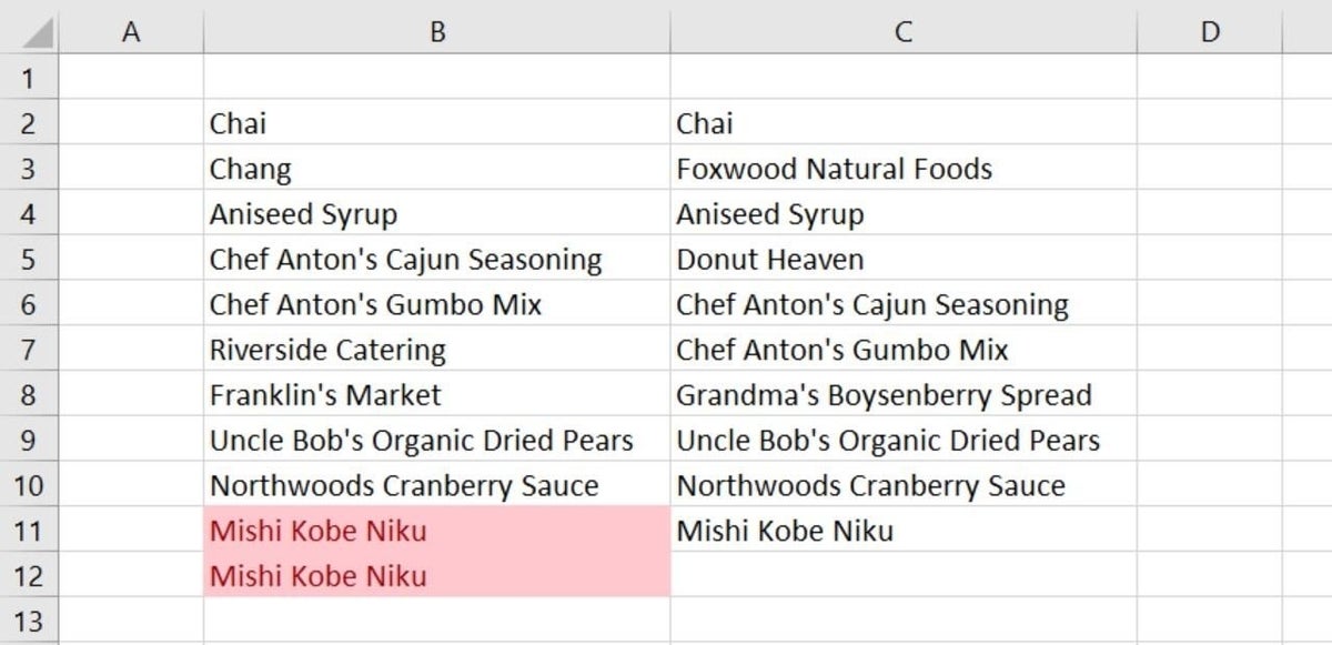
The built-in rules highlights duplicates in the same column.
Now let’s use the same built-in rule to compare the list in columns B to the list in column C. To do so, select B2:C12 and follow the same steps as above. Figure C shows the results. This rule applies highlighting if the item appears more than once–anywhere. That might include duplicates in the same column or items that occur more than once across both columns.
Figure C
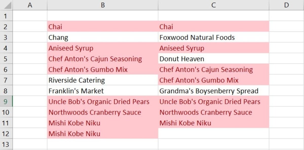
The duplicate rule highlights any item that occurs more than once in the selected range.
See: 10 Excel time-savers you might not know about (TechRepublic)
Custom rules
The two lists shown in Figure A are similar, but there are subtle differences. A few items are unique to both lists. In addition, sometimes the item in column B differs from the corresponding item in column C. In this section we’ll use a custom conditional formatting rule to spot the items that are different from one column to the other. You can think of these items as mismatched. We’ve already seen that the built-in rule evaluates all values in any position, and that’s not what we want.
Conditional formatting can quickly identify differences between two lists–from column to column–using an expression in the form:
=COUNTIF(otherlist,firstcellinselectedlist) = 0
Now, let’s apply this rule to column B as follows:
- Select the list in column B, B2:B12.
- Click the Home tab, click Conditional Formatting in the Styles group, and choose New Rule from the dropdown list.
- Choose the Use a formula to determine which cells to format option.
- Enter =COUNTIF(C2:C2,B2)=0 in the Formula control.
- Click Format, click the Fill tab, choose a color, and click OK. Figure D shows the format and the rule.
- Click OK to return to the sheet shown in Figure E.
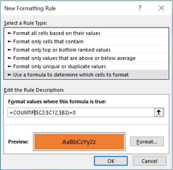
Figure D
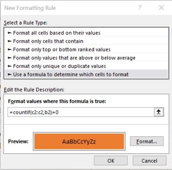
This rule will highlight items in column B that don’t match the corresponding items in column C.
Figure E
The highlighted items in column B don’t match the corresponding value in column C.
This rule doesn’t highlight duplicates; any value in column B that contains a value not in the corresponding cell in column C is easy to identify thanks to the cell’s contrasting fill color. It doesn’t highlight values that occur in both columns as the built-in rule did. To apply the rule to column B instead, you’d use the rule =COUNTIF(B2:B2,C2)=0 after selecting C2:C11.
This rule works with values as well as text entries. The lists don’t have to match in size either. For example, the rule highlights the last value, Mishi Kobe Niku because the corresponding cell in column C is blank. In addition, slight differences matter. For instance, if you remove the apostrophe character in Bob’s, the items no longer match. On the other hand, the comparison isn’t case sensitive. If the format doesn’t highlight an item as you expect, compare the two items. It’s possible there’s an additional space character.
Next, we’ll use the same technique with a slightly different reference to compare two lists; if an item in column B doesn’t occur anywhere in column C, highlight that item in column B. Earlier, we highlighted mismatched items from column to column; now we’re going to highlight unmatched items in both columns.
In this example, we’ll highlight items in column B that don’t occur in column C, as follows:
- Highlight B2:B12.
- Click the Home tab, click Conditional Formatting in the Styles group, and choose New Rule from the dropdown list.
- Choose the Use a formula to determine which cells to format option.
- Enter =COUNTIF($C$2:$C$12,$B2)=0 in the formula control.
- Click Format, click the Fill tab, choose a color, and click OK. Figure F shows the format and the rule.
- Click OK to return to the sheet shown in Figure G.
Figure F
This rule will highlight items in column B that don’t occur anywhere in column C.
Figure G
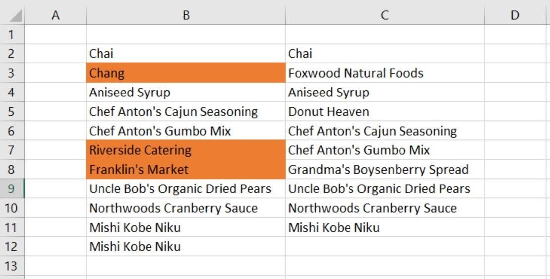
Any value in column B that doesn’t occur in column C is easy to identify thanks to the cell’s contrasting fill color.
As you can see, there are three items in column B that don’t occur in column C. But what about column C? To identify items in column C that don’t occur in column B, repeat the above steps. However, in step 1, select C2:C12 and in step 4, enter the formula =COUNTIF($B$2:$B$12,$C2)=0; choose another color in step 5, if you prefer. As you can see in Figure H, four items in column C, including the blank at C12, don’t occur in column B.
Figure H
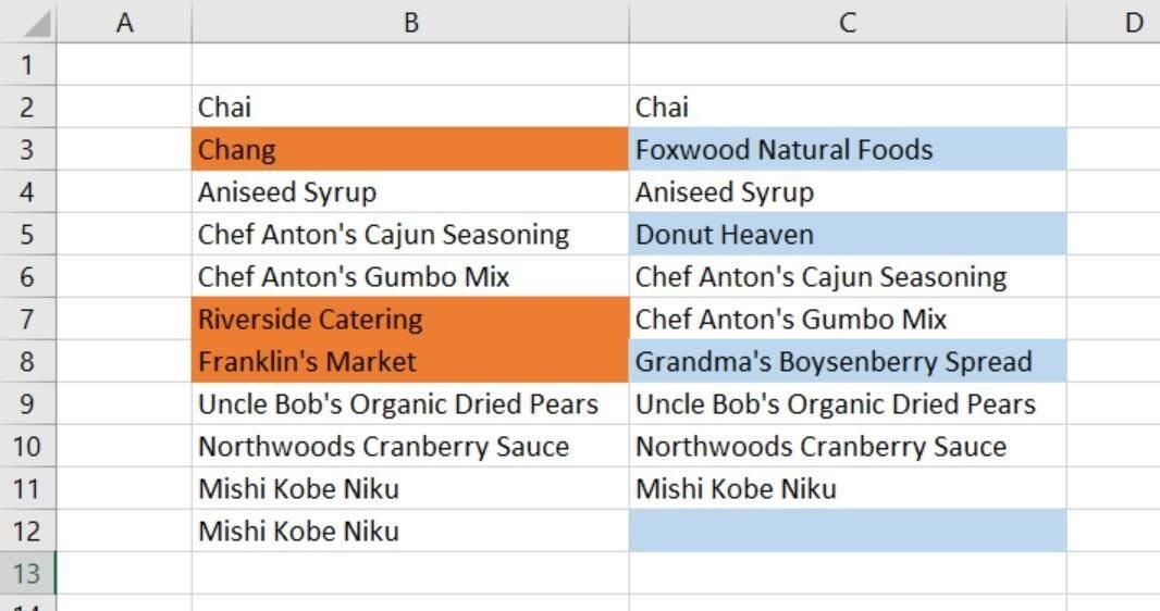
Two similar rules highlight items that don’t occur anywhere in the other list (column).
Stay tuned
In a subsequent article, we’ll continue with more complicated duplicate-finding problems.
Send me your question about Office
I answer readers’ questions when I can, but there’s no guarantee. Don’t send files unless requested; initial requests for help that arrive with attached files will be deleted unread. You can send screenshots of your data to help clarify your question. When contacting me, be as specific as possible. For example, “Please troubleshoot my workbook and fix what’s wrong” probably won’t get a response, but “Can you tell me why this formula isn’t returning the expected results?” might. Please mention the app and version that you’re using. I’m not reimbursed by TechRepublic for my time or expertise when helping readers, nor do I ask for a fee from readers I help. You can contact me at susansalesharkins@gmail.com.
Also see:
- How to apply an Excel validation control that protects a specific limit (TechRepublic)
- How to create transparent text in PowerPoint 2016 (TechRepublic)
- How to create a quick and easy online form with 365 Microsoft Forms (TechRepublic)
- How to build a simple timesheet in Excel 2016 (TechRepublic)
-
You’ve been using Excel wrong all along (and that’s OK) (ZDNet)