Image: iStock/panimoni
Microsoft Excel’s Find feature is one of its most flexible tools in the entire toolbox. You can do much more than just find and replace data. For instance, you can use it to apply or delete formatting, insert new text without removing the find text, apply or delete a style, transpose data, and much more. In this article, I’m going to show you how to use Find to select values and then manipulate them in some way, but we’ll go a step further by deleting individual instances of the found values before we do anything to them. That’s something you can’t do quickly with Find & Replace or a filter.
SEE: 60 Excel tips every user should master (TechRepublic)
I’m using Microsoft 365 on a Windows 10 64-bit system, but you can use earlier versions. You can work with your own data or download the demonstration .xlxs file. The browser edition supports the Find All list, which is the basis for this article. Unfortunately, you can’t delete items from the list in the browser, which means Find All is limited in the browser.
How to select cells using Find All in Excel
Selecting cells that contain specific values is probably a familiar task using Find, but I’m going to show you some options that you might not regularly use. First, you need to determine whether you want to search the entire sheet or a range—we’ll work within a range as follows:
- Using the data shown in Figure A, select A2:D13. If you want to search the entire sheet, click any cell on the current sheet but limiting the range will make what we plan to do easier.
- Press Ctrl+F to open the Find dialog. Or, on the Home tab, select Find from the Find & Select option in the Editing group.
- To find all the cells that contain James, enter James in the Find What control.
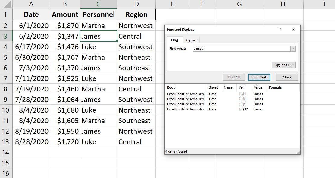
- Click Find All, and Excel will display a list of all instances of James. If you click Find Next, Excel will select the first instance of James—don’t do that right now. (Enlarge the Find and Replace dialog if necessary.)
Figure A

Excel selects the first instance in the selected range in the list and in the sheet (Figure A). By selecting another instance in the list, you can move the sheet selection accordingly. This method gives you a bit more control than Find Next because you don’t have to browse all of the instances; you get to choose. There’s a lot more you can do via this list, though. Let’s take a look at some of the things you can do.
How to apply formatting in Excel
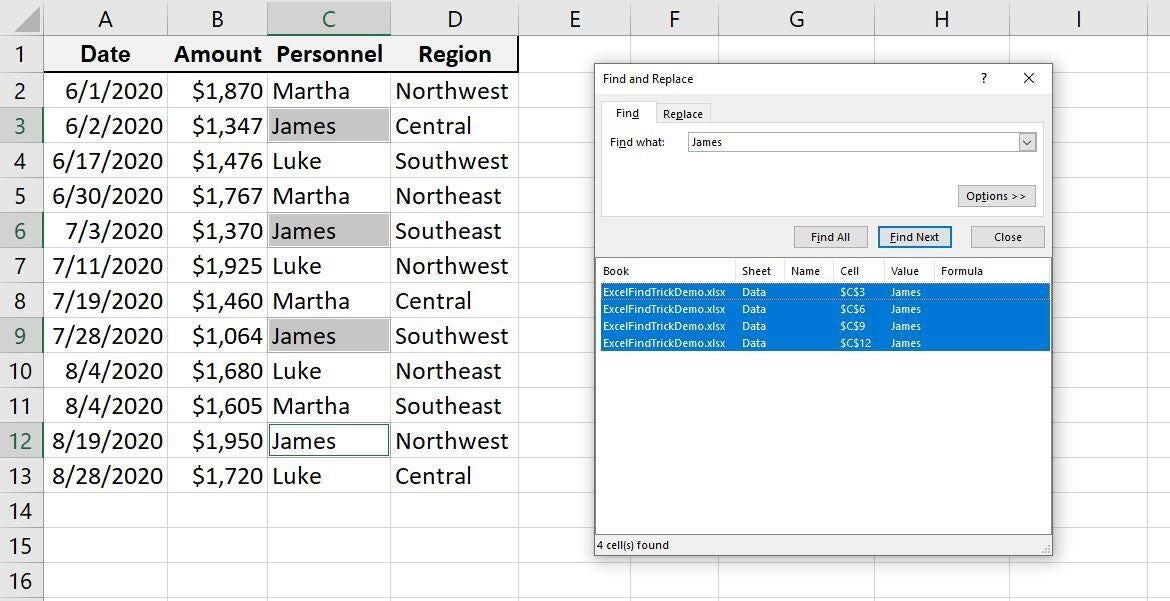
One of the easiest things you can accomplish using this Find All feature is highlighting all the found instances of your search string—in our case, that’s James—so you can do something to or with those cells. First, press Ctrl+A to select all instances of James, as shown in Figure B.
Figure B

With all those cells selected, you can do many things. For example, choose a color from the Fill Color palette in the Font group (on the Home tab.) Figure C shows the results of choosing light orange.
Figure C

You can do the same thing using Find and Replace, but you have to use Find Next to browse though the entire selection if you don’t want to apply the format to them all. Using the Find All list, you can avoid that tedious route. By deleting items from the list, you can focus on a subset of the cells containing James as follows:
- In the list, select the third item—cell $C$9—and press Delete. Excel will remove it from the list, and you’re left with a list of 3. Doing so deletes items from the list; it will not delete the value in the sheet.
- Press Ctrl+A to select the three items in the list.
- In the Font group, click Italics. The results are shown in Figure D.
Figure D

So far, we’ve used Find to do a few simple things. Let’s use it to do something a bit more powerful.
How to delete rows with Find in Excel
It might have occurred to you at this point, that this feature might provide a quick way to delete cell values and even records. It isn’t the only way, but it is quick and has an advantage over Excel’s filtering feature, which will also delete rows. Using Find, you can remove any instance from the delete task, but using the filtering feature, you can’t. You can use more filters to reduce the number of matches, but you’re still filtering, which may or may not give you the same results as Find.
SEE: How to calculate bonuses and commissions in Excel (TechRepublic)
Before we continue, it’s important to note that deleting a row can have consequences you didn’t count on. Specifically, you might delete data that’s off screen and forgotten. Even selecting the data set first, as we did, won’t protect that data. However, remember that you can press Ctrl+Z to undo a delete preformed this way.
Now let’s return to the list and delete the rows containing James as follows:
- In the list, press Ctrl+A to select all the instances.
- In the Cells group (on the Editing tab), click Delete and choose Delete Sheet Rows.
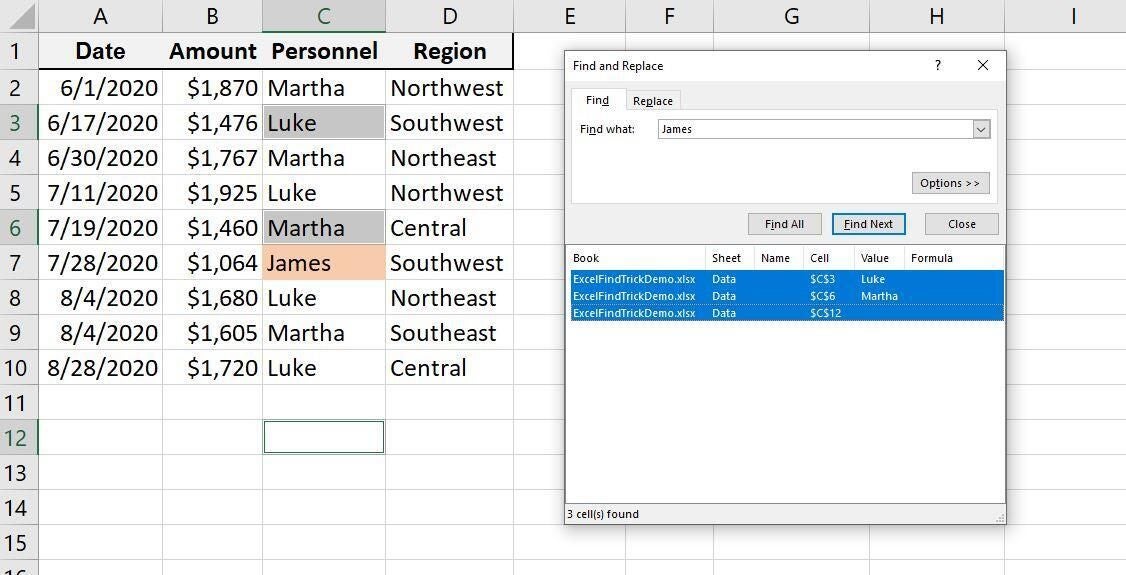
If you were expecting to delete all four rows, you might be surprised. As you can see in Figure E, the task missed one (row 7). Remember when we deleted the item for cell C9 in the list earlier? That instance of James is now in row 7 because the delete task deleted two rows above row 9. That may or may not be want you want to do, but now you can see the possibilities, or flaws, depending on what you intended to do.
Figure E

More options to try in Excel
You can combine the list with other options, but we didn’t touch on those. For instance, you might want to select all the cells that contain formulas. By selecting Formulas from the Look in control (click Options), you can select all formula cells and then remove instances. You can also select all formula cells using Find and Select, but you can’t easily remove cells from the resulting selection. Keep this feature in mind when you have tasks that filtering and other selection methods can’t adequately handle.

