


Image: iStock/AndreyPopov
Must-read Windows coverage
- CrowdStrike Outage Disrupts Microsoft Systems Worldwide
- 10 Best Project Management Software for Windows in 2024
- Windows 10 Extended Security Updates Promised for Small Businesses and Home Users
- Securing Windows Policy
If you’ve ever had a job that earns a commission, you know how difficult it can be to calculate. A flat commission pays the same rate, regardless of the total. For example, if the rate is 2%, you make 2% whether your totals are $1,000 or $1,000,000. A tiered commission (usually) encourages sales, because the better you perform, the higher the percentage.
In this article, we’re going to build a simple tiered system in Microsoft Excel that changes the rate based on the total. Each milestone raises the rate. Although we’re using the term commission, you can use the same structure for bonuses. It’s the best place to start when tackling tiered systems, and it won’t require any acetaminophen.
SEE: 60 Excel tips every user should master (TechRepublic)
I’m using Microsoft 365 on a Windows 10 64-bit system, but you can work in earlier versions. For your convenience, you can download the demonstration .xlsx file. This solution is compatible with the web version.
The simplest hierarchy
The simplest tiered hierarchy might not be a true tiered system at all in accounting terms, but we’re going to treat it as such. For instance, let’s suppose the first rate of 2% is paid on totals up to $50,000. Sales over $50,000 receive 2.5%, and totals over $80,000 receive 3%. It’s important to note at this point that the percentage is paid on all totals once the benchmark is met—that’s why some might not consider this a true tiered system.
SEE: Windows 10: Lists of vocal commands for speech recognition and dictation (free PDF) (TechRepublic)
The business rules are applied by the company paying the commissions. There will never be one rule for them all. It isn’t difficult, but you must know the rules to set this up. For that reason, I want to encourage you to work dynamically so you can easily update when milestone and percentage values change.
If you’re stressed by the thought of coming up with a set of unique expressions that represent your organization’s tier system, don’t worry. Start by writing them out in words, so everyone is on the same page Here are the tiered system rules that we’re going to apply in this simple demonstration:
- Monthly totals under $50,000 are multiplied by .02; $50,000 is the first milestone.
- Monthly totals under $80,000 are multiplied by .025; $80,000 is the second milestone.
- Monthly totals over $80,000 are multiplied by .03; with only three tiers, there isn’t a third milestone.
Once you break it down in this way, the expressions are much easier to discern. Now, let’s get started.
How to create a tier table
My first bit of advice is to not enter the milestone and percentage values into your expressions. Instead, create input cells and reference those. That way, you can easily adapt the sheet when milestone and percentage values go up (or, unfortunately, down).
SEE: Tech budgets 2021: A CXO’s Guide (free PDF) (TechRepublic)
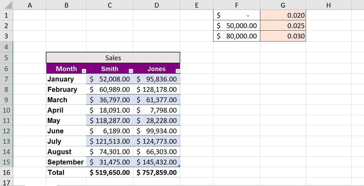
As you can see in Figure A, I’ve created a simple tier table that reflects the rates from the previous section. (The sheet in Figure A is simple on purpose.) Apply the accounting format to F1:F3 and the number format to G1:G3. You might want to build the commission table on another sheet, but I’m showing it all on one sheet so you can see the solution and the original data together. Our next step is to add the expressions that combine the data and the tier table to return monthly commissions for all personnel. That’s why the tier table is offset a bit.
Figure A
How to create the expression to calculate commissions
If you search for tiered commission solutions, you might feel a bit stymied and want to give up. In our case, the solution is much simpler than most of what you’ll find. That’s not because I’m so brilliant; rather, we are looking at a simple problem. Simply put, we need an expression that compares the monthly total to the nearest milestone value in column F of the tier table and returns the corresponding rate in column G. A VLOOKUP() function can do that. Then, it’s simply a matter of multiplying that rate by the monthly total.
First, we need a new table. Figure B shows a matching Table object with no data or expressions. Simply copy the Table and remove the data. Enter the following expression into G7 (the commission table) and copy to fill the remaining data range (G7:H15):
=VLOOKUP(C7,$F$1:$G$3,2)*C7
The commissions, like magic, populate the commission table, as you can see in Figure C.
Figure B
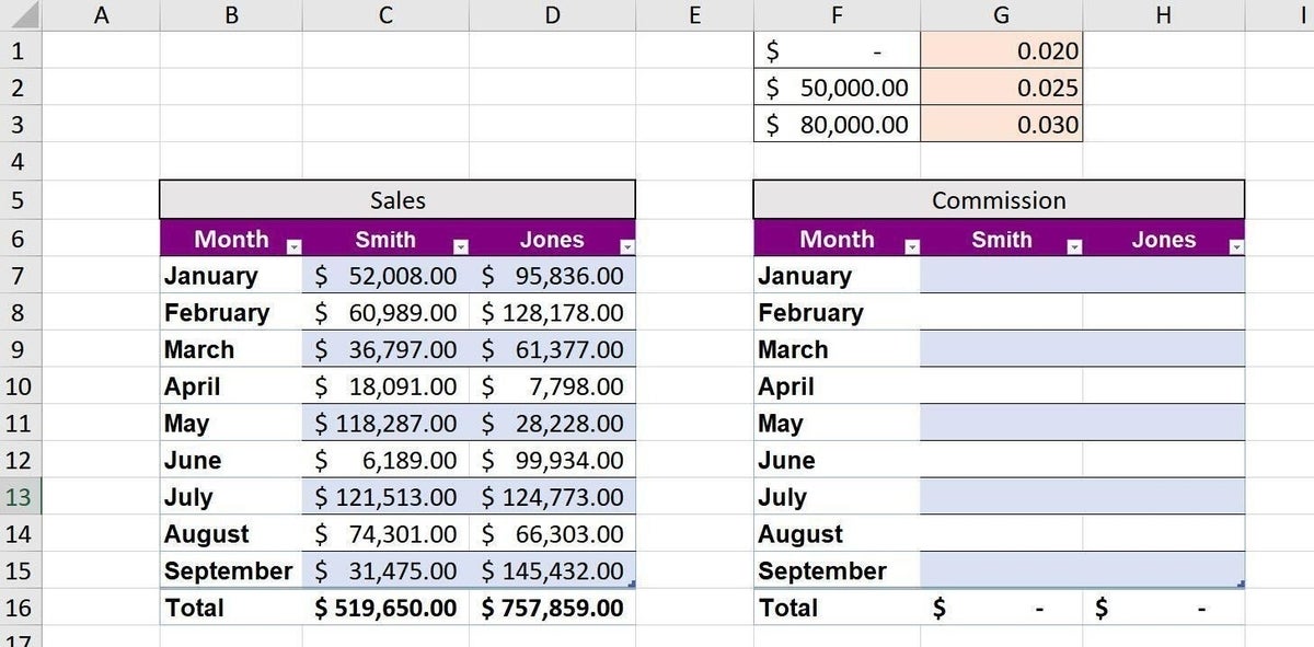
Figure C
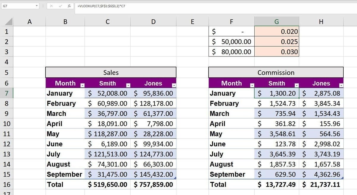
Let’s pick apart the expression. First, the VLOOKUP() function compares a monthly total in the sales table, $52,008 (in C7). The nature of this function helps us because it doesn’t have to find an exact match, and it keeps evaluating the list until encountering a value that’s greater than the original value. In this case, that’s $80,000—80000>52008. The argument 2, tells the function to go over 1 column from the milestones in column F and return that value, which is .025. The final part of the expression multiplies .025 by $52,008 to return $1,300.20.
Now, let’s break it down as an expression:
=VLOOKUP(52008,$F$1:$G$3,2)*C7=
=VLOOKUP(52008,{0,0.02;50000,0.025;80000,0.03},2)*C7=
=0.025*52008=
=1300.20
SEE: How to use sheet view for more flexible collaboration in Excel (TechRepublic)
How to change commissions in the Excel table
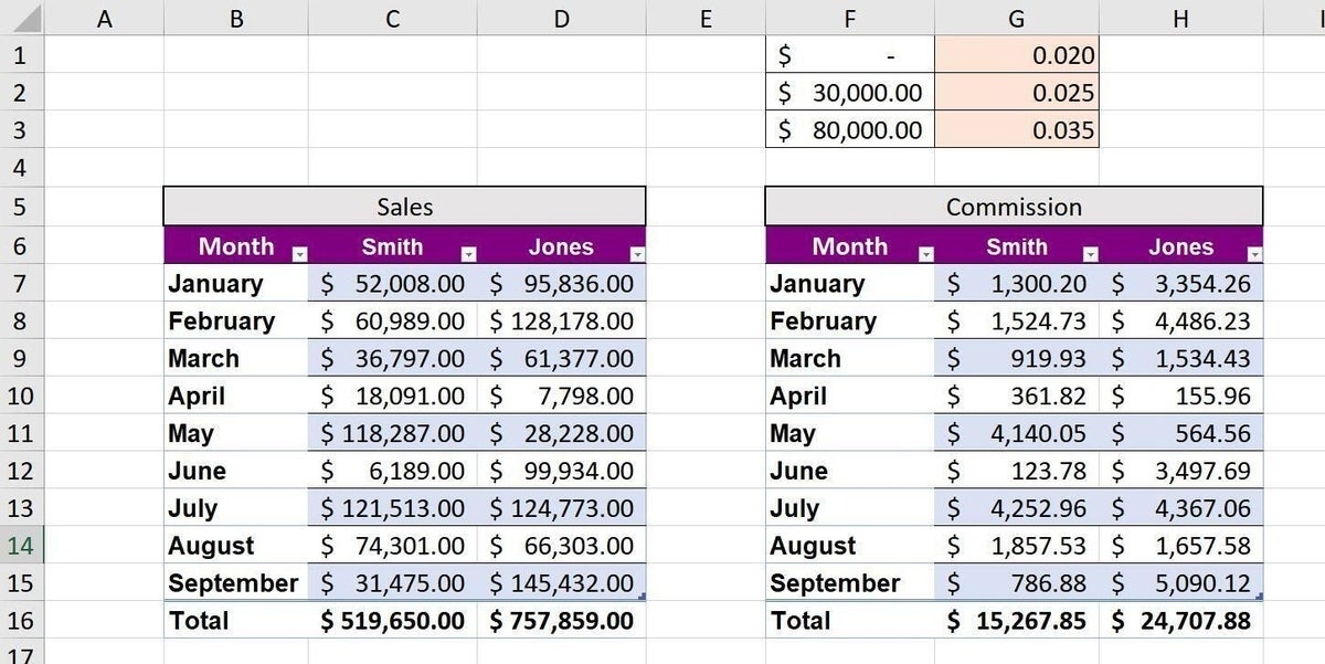
Because the milestones and percentages are input cells, you can quickly update all commissions, by simply changing the values in the tier table, as shown in Figure D. Rates went up a bit! By changing one value or all of them, you can update the commissions owed immediately. When changing these values, remember that the milestone values in column F must be in ascending order. In addition, the table objects accommodate new rows in both table objects automatically.
Figure D
Stay tuned
This solution turns out to be simpler than you might think. If you were expecting a complex and convoluted expression, I’m glad to be able to surprise you. This easy solution barely touches the surface on the topic of tiered commission system though. In a subsequent article, we’ll make things a bit tougher.