


One of the reasons Microsoft Excel is so popular for so many tasks that aren’t necessarily financial or arithmetical is the many options for converting, transforming, cleaning up, enriching and generally wrangling raw data into the right shape to use. The Power Query technology in Excel (now known as Get & Transform) is so good at data transformation that it’s what the Power BI desktop app is based on, so you can repeatably pre-process data for analytics, visualisation and even machine learning.
SEE: Software Installation Policy (TechRepublic Premium)
More about Software
- Software Installation Policy
- Five Methods to Insert a Checkmark Into Microsoft Office Products
- How to Hide and Handle Zero Values in an Excel Chart
- How to Use Section Breaks to Control Formatting in Word
You don’t have to connect to external data sources to find the various data transformation tools in Excel useful. If you need to massage the responses from online forms and questionnaires, clean up an address list, strip out punctuation and HTML tags from data copied from online sources or reformat your credit card statements so you can copy the transactions into your expense claim, Excel is the perfect tool. You can also make sure dates and currency amounts are formatted correctly or add extra data like the exchange rate (the XLOOKUP function added in 2019 is ideal for that).
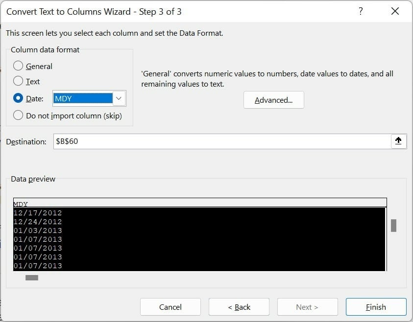
The Text-to-Columns feature (find it under Data, Data Tools) does a lot more than the name would suggest. Opening a spreadsheet with dates in U.S. format? You could laboriously create a second volume and create a complex formula to reverse the day and month order to get UK format dates: or you could use the Text-to-Columns wizard to switch them all for you. Select the cells with the U.S. format dates in, choose Delimited on the first screen of the wizard then clear all the suggested Delimiters on the second screen. On the third screen, set the Date format to MDY. The preview may still look wrong but when you click Finish, the dates will be in the right format.
Text to Columns can also split apart text into multiple cells: handy for discarding extra information like the merchant number on a credit card transaction or moving the postal code to a separate field so you can sort addresses by location. If you want to do that automatically on hundreds of spreadsheets without creating a data pipeline using the Get & Transform tools, a formula can be a better approach than a dialog you have to click through. You could combine the SEARCH, FIND, LEFT, RIGHT, MID, LEN, SUBSTITUTE and SEQUENCE functions to break apart text using delimiters like commas or even the spaces between words, but you end up writing complicated regular expressions.
SEE: Why Microsoft Lists is the new Excel (TechRepublic)
The latest Office Insider betas for Microsoft 365 subscribers add new functions that act like the Text-to-Columns wizard. TEXTSPLIT breaks the text in a cell up into multiple cells (one for each delimiter): the first value you give the function is the cell with your data in. You can split text across columns or into multiple rows if you want to turn a paragraph of text into individual sentences by specifying the column or row delimiters. These are the second and third values in the function, and you need to put quotes around the delimiter character – like “,” for a comma or “=” for the equals symbol. If you want TEXTSPLIT to deal with multiple delimiters the same way, list them as an array: TEXTSPLIT(A1,{“,”,”;”}) will break up text that is separated by both commas and semicolons.
Or you can turn your text into an array (in Excel that’s a table that isn’t formatted as a table) by telling TEXTSPLIT about delimiters for both rows and columns.
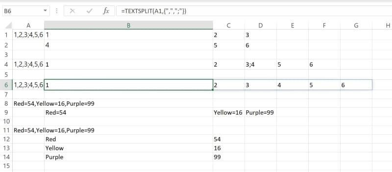
If you start with the data Red=54,Yellow=16,Purple=99 in cell A1, TEXTSPLIT(A1,”,”) will create three new cells with Red=54 in the first, Yellow=16 in the next and Purple=99 in the third. TEXTSPLIT uses dynamic arrays so the text spills into as many cells as necessary (you’ll get an error if the spilled array would overwrite a cell that already has data in, to make sure you don’t lose data without realising).
If you need to always have the same number of columns or rows even when there isn’t the same amount of data, you can tell TEXTPLIT to create empty cells if there are two delimiters side by side with no value in between. By default, TEXTSPLIT ignores the empty value but put TRUE as the fourth value in the function and it will add in empty cells.
If you want to copy just part of the text out of a cell, use TEXTBEFORE and TEXTAFTER: You specify the delimiter in the same way, but you also say which item from the list you want (1 gives you the first item, 2 the second or -1 the last and -2 the second to last). The difference between the two functions is whether you get the text before or after the delimiter. This is particularly powerful because the delimiter doesn’t have to be the usual punctuation marks; you can use text as the marker for where to start copying–or use a space to split names into first and last names.
When you have data arranged by columns and you want it in rows (or vice versa) you can copy and then paste transpose to rearrange it. New functions for changing the shape of data let you do that with a formula instead: TOROW turns an array into a single row, TOCOL turns it into a single column and WRAPROWS and WRAPCOLS turn rows and columns into arrays.
You can also join two arrays by using VSTACK and HSTACK to stack them one below the other or side by side, removing any empty cells between them. And if your content is already in multiple cells, there’s a set of functions that let you grab columns and rows out of an array either by specifying the columns and rows you want (CHOOSEROWS and CHOOSECOLS) or by saying which rows and columns you want to keep (TAKE) or ignore (DROP), starting from the beginning or end of the array.
Excel already lets you target columns in tables fairly easily, but working with arrays hasn’t been as easy and now that any formula that returns multiple results spills them into a dynamic array of cells, having functions to target columns and rows inside those arrays is very useful.
Auto lists
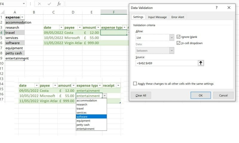
If you’re entering text and you want to make sure you’re consistent about things like product names, accounting categories, abbreviations for states in addresses or anything else where you’re effectively selecting from a list of possibilities, you can create a dropdown list in Excel by choosing Data, Data Validation and choosing List in the Allow box on the Settings tab. Use a table on your spreadsheet for what will be shown in the list so you can easily expand it: you can put that on a different tab and select it in the Source box (hide or lock the tab if you don’t want people to be able to change what’s in the list).
But that gets unwieldy when you have hundreds or thousands of entries on the list that people have to scroll through or type in perfectly. You can add a combo box form control that lets people start typing and have Excel fill in the cell with entries from the list that match what they’re typing, but that’s no longer a standard cell (and you have to create a combo box everywhere you want to use the list rather than just using AutoFill to add the dropdown list to every cell in the column).
This is such a common request that there are Excel extensions to do it, and Microsoft is finally adding AutoComplete for dropdown lists. You don’t have to do anything different: Make your dropdown list as normal using the Data Validation feature and once you click to open the list you can start typing to filter the list. If there’s a single match, that will be autocompleted; if there are a few, it’s still a lot less to choose from.
As with all features in Office Insider betas, these features may change or even go away before they’re fully released; dropdown AutoComplete has already been pulled, rewritten and rereleased, changing in April from letting you select the cell and start typing to having to open the dropdown list before you start typing. That’s caused some frustration, as has the fact that even if you have the latest version of Office Insider you may not see it in your build because of the way Microsoft flights Office features.
A new feature is released to a subset of users; if telemetry shows it doesn’t cause crashes, performance problems or other issues it will then be progressively released to more users. These tranches are often done across all users rather than turning on features for everyone in an organisation or on an Office 365 tenant, because that lets Microsoft test on the widest range of hardware and software configurations, network topologies, bandwidth and so on. (File, Account, What’s New should show if the feature is enabled for you but it’s a long list of features that you can’t easily search and the dialog box for creating dropdown lists doesn’t look any different if you have the new feature.)
If that’s frustrating (or confusing to your users), make sure they’re not using beta releases (which are unsupported and only designed for test environments). The Current Channel (Preview) includes features that will be in the next release so you can let users try them out early and still be supported–but it’s still not guaranteed that everyone using an Office Insider build will get the new features at the same time, so warn people that this tends to be unpredictable.