


LAMBDA functions are new to Microsoft Excel. With LAMBDA functions, you can turn a complex calculation into a simple sheet-level function. You must know the complex calculation, but those are prone to errors and difficult to maintain; for instance, if something changes, you might end up altering several sheet-level formulas. Why not use a LAMBDA() instead? You enter the complex calculation once, give it a function name, and that’s it.
In this tutorial, I explain what a LAMBDA function is and how to use Excel’s new LAMBDA() function. I assume you have at least basic Excel skills. Once you learn how to use LAMBDA functions, expect to use them a lot in your Excel spreadsheets.
SEE: Software Installation Policy (TechRepublic Premium)
I’m using Microsoft 365 on a Windows 10 64-bit system. Excel’s LAMBDA() function is available only in Microsoft 365 and Excel for the Web. I assume you have basic Excel skills. For your convenience, you can download the demonstration .xlsx file. This article assumes you have basic Excel skills, but you should be able to follow the instructions to success.
What is a LAMBDA() function?
Must-read Windows coverage
- CrowdStrike Outage Disrupts Microsoft Systems Worldwide
- 10 Best Project Management Software for Windows in 2024
- Windows 10 Extended Security Updates Promised for Small Businesses and Home Users
- Securing Windows Policy
An Excel LAMBDA() function is similar to a VBA user-defined function – without VBA. In short, Excel’s LAMBDA() lets you create custom and reusable functions and give them meaningful names using the form:
LAMBDA([parameter1, parameter2, …,] calculation)
where the optional parameter arguments are values that you pass to the function—arguments can also reference a range. The calculation argument is the logic you want to execute. Once all that’s correct, you save it all by using Excel’s Name Manager to give it a name. To use the function, you simply enter the function name at the sheet level, as you would any of Excel’s built-in functions.
That’s all great, but there’s more. Excel LAMBDA() supports arrays as arguments, and they can also return results as data types and arrays. The average user might not need this much power, but you should know it’s available.
Before we continue, there are a few rules you must abide by when creating a LAMBDA() function:
- LAMBDA() supports 253 parameters, which should be plenty for most users.
- LAMBDA() follows Excel’s name and parameter name conventions, with only one exception: You can’t use the period (.) character.
- Like other functions, LAMBDA() will return an error value, if appropriate.
How to create a LAMBDA() function in Excel
Creating a LAMBDA() function in Excel is fairly simple. Using LAMBDA(), you enter the parameters and calculation arguments using variables. Using Excel’s Define Names feature, you name the function and enter the LAMBDA() function, and that’s it.
The easiest way to understand what Excel’s LAMBDA() functions can do for you is to start with a simple one. For example, Excel offers a SUM() function but not a SUBTRACT() function. You can still subtract, but it’s a simple calculation to begin with:
- Enter the test calculation =B3-C3 into any cell outside the Table. If it returns the expected results, continue. If not, keep working on the calculation until it’s correct.
- Click the Formulas tab and then click Define Name.
- In the resulting dialog, enter SUBTRACTYL in the Name control. The L suffix identifies the function as a LAMBDA() function, but you can use any convention you like.
- For now, don’t change the Scope setting, but you can limit LAMBDA() to a sheet instead of the workbook.
- Enter a comment that describes the LAMBDA() function, such as Subtracts two numbers.
- In the Refers to control, enter the LAMBDA() function, =LAMBDA(a,b,a-b) (Figure A).
- Click OK.
Figure A
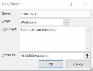
The variables a and b first identify the values being evaluated and a-b is the calculation. Because there are only two variables, SUBTRACTL evaluates only two values or two ranges.
At this point, you’re ready to use the LAMBDA() function SUBTRACTL().
SEE: Python programming language: This training will jump-start your coding career (TechRepublic Academy)
How to call an Excel LAMBDA() function
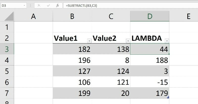
You’ll use LAMBDA() functions the same way you use Excel functions. To demonstrate, enter the function and reference the values shown in Figure B, =SUBTRACTL(B3,C3). (The period is grammatical and not part of the function.) B3 and C3 satisfy the variables a and b, respectively. The calculation subtracts b from a, in the order specified at the function level.
Figure B
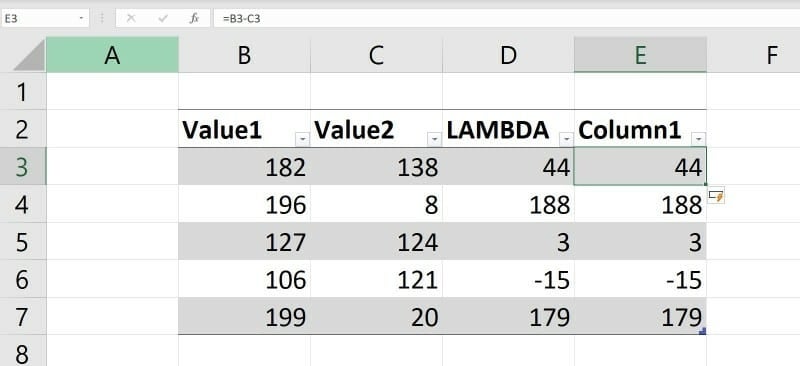
When working with a new LAMBDA(), you can check it by dropping in the original formula. In this case, that’s =B3-C3. As you can see in Figure C, the checking expression and the LAMBDA() return the same results. Even though you checked the calculation before you created SUBTRACTL(), it’s a good idea to test again. If you’re using a Table object (as I am), Excel uses structured referencing, =[@Value1]-[@Value2].
Figure C
It’s worth mentioning that you can always explicitly pass the values. For example, the function SUBTRACTL(182,138) returns 44.
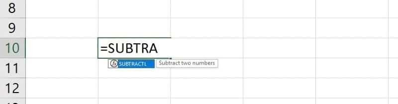
Because Excel’s LAMBDA() uses Excel’s formula language, it behaves predictably. For instance, when you start to enter the function by entering only a few characters, SUBTRACTL() pops up in the AutoComplete list, as shown in Figure D. Notice that Excel also displays the description that you entered when you named it. The one thing it can’t do, as yet is show the arguments as a built-in function would.
Figure D
Before we look at a more reasonable and complex LAMBDA(), let’s review a few errors that you might experience with their use.
About Excel LAMBDA() errors
LAMBDA() functions are as prone to errors as built-in functions. You must pass the expected parameters, and the calculation logic must be sound. Otherwise, you could see errors. Let’s look at some of the possibilities:
- #VALUE!: If you see this error value, check your passed arguments—you passed the wrong number.
- #NUM!: Check for a circular reference if you see this error value.
- #NAME!: Check the actual function name you entered for a typo.
For most of us, the #VALUE! Is the most likely to occur, and it’s easy to troubleshoot. Now, let’s look at a more complex LAMBDA().
SEE: Why Microsoft Lists is the new Excel (TechRepublic)
How to use Excel LAMBDA() to return top n values
You’ve learned a lot, and now it’s time to use what you’ve learned to create a useful LAMBDA(). Calculating the top n values in a column is a common task and requires a bit of specialized knowledge. In the past, you could use an advanced filter, an expression or a PivotTable. In addition, you could use a conditional formatting rule to highlight those values at the source. The article, How to return the top or bottom n records without a filter or PivotTable in Excel uses none of those and relies on Excel’s array functions, SORT() and SEQUENCE().
Now we’ll tackle the problem using Excel’s LAMBDA() function. We’ll also use Excel’s SEQUENCE() array function in the form
=LAMBDA(values, n, LARGE(values, SEQUENCE(n)))
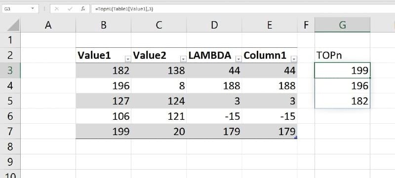
Figure E shows the above function in G3. You can tell it’s an array function because the results have a blue border. Let’s break it down so you can see how it works:
- When entering the function, select the Value1 values—don’t include the header cell. Doing so satisfies the values argument.
- Enter 3, satisfying the n argument.
- SEQUENCE(n) is an array function that determines the number of rows to return, but in this case, it’s numbers from Table1[Value1].
- The LARGE() function is an Excel built-in function that returns the nth largest value in a range.
Figure E
The LAMBDA() passes the reference of the numbers you want to evaluate (values) and the number you want the array to return (n). The calculation portion, LARGE(values, SEQUENCE(n)) does the work, but the LAMBDA() makes it easy to use. This is one of the grand things about LAMBDA() functions—users don’t need specialized knowledge to get their work down.
Now that you know how it works, let’s create it:
- Click the Formulas tab and then click Define Name.
- In the resulting dialog, enter TOPnL in the Name control. The L suffix identifies the function as a LAMBDA() function, but you can use any convention you like.
- For now, don’t change the Scope setting, but you can limit the LAMBDA() to a sheet.
- Enter a comment that describes the LAMBDA() function, such as Returns the top n values as a LAMBDA().
- In the Refers to control, enter the LAMBDA() function, =LAMBDA(values, n, LARGE(values, SEQUENCE(n))). (Figure F).
- Click OK.
Figure F

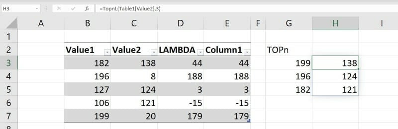
After entering TOPnL() in G3 (Figure E), copy it to H3 and see what happens. The reference is relative so you get a second array of the top three values in Value2, as you can see in Figure G.
Figure G
For more on the subject of returning the top n values, read these TechRepublic articles: