


If you work with transaction records, you probably need a way to track what’s outstanding and what’s been paid. At any given time, you might want to know how much a specific customer owes, how much all of your customers owe, or even how many payments you’ve received. There are many ways to analyze transaction records; in this article, I’ll show you three ways to match or reconcile transaction: using functions, the Subtotal feature, and a PivotTable.
More about Software
- Software Installation Policy
- Five Methods to Insert a Checkmark Into Microsoft Office Products
- How to Hide and Handle Zero Values in an Excel Chart
- How to Use Section Breaks to Control Formatting in Word
Transactions don’t have to be monetary; you could just as easily be tracking rental equipment. But any time there’s a transaction, you will eventually need to reconcile both ends of that exchange–what went out, what came in. We’ll use the terms match and reconcile loosely to describe what we’re doing because nothing in this article resembles a professional receivable program. Rather, I’ll show you how to use built-in tools to group and analyze your transaction records to provide temporary and on-the-spot meaningful information.
I’m using Excel 2016 on a Windows 10 64-bit system. You can apply this article to earlier versions, but the steps will differ. The functions and PivotTable work easily in the browser. Although the browser will display subtotals in an existing sheet, you can’t use the browser to apply the feature. You can work with your own data or download the demonstration .xlsx and .xls files.
SEE: How to use Excel’s what-if tools to analyze business scenarios (free PDF) (TechRepublic)
Functions
The data in Figure A is very similar to what you might see in a database table; it’s certainly not a typical spreadsheet. This record-type construct has pros and cons. It’s great for storing and analyzing, but not so great for reporting.
Figure A
This data set resembles a database record, not a traditional spreadsheet.
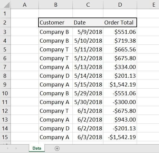
Currently, we have a nice list of invoice totals and payments; we have records for money owed and money paid. That’s it. Given the current structure, there’s no easy way to determine which customers owe us money. Your first thought might be to generate a quick matrix using a simple SUMIF() function, as shown in Figure B:
=SUMIF($B$3:$B$15,"="&H$2,$D$3:$D$15)
Unfortunately, if you add rows to the data set, the SUMIF() functions won’t update. An easy fix would be to convert the data set to a Table object; then the matrix will update as you add new records.
Figure B
A simple SUMIF() returns totals for each company.
The second problem is that you can’t limit the SUMIF() results by date, which would be a reasonable expectation with this type of data. You could use a SUMIFS() in the matrix and reference dates, but that will quickly grow unwieldy.
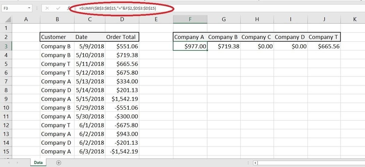
You could just as easily add a function adjacent to the data set, as shown in Figure C. Either of the following functions will work:
=SUMIFS($D$3:D$15,B$3:B$15,$B3)

=SUMIF($B$3:$B$15,"="&B3,$D$3:$D$15)
Figure C
Return the outstanding amount for each company adjacent to the data set.
This route repeats results because you’re summing by customer (column B). If that’s not distinct enough, there’s one more function you can try:
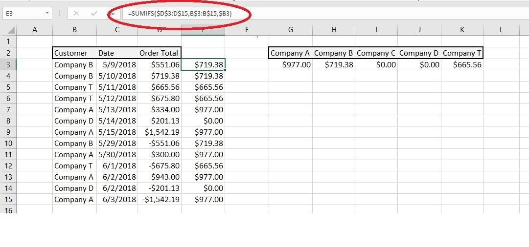
=ROUND(SUMIF($B$3:$B$15,"="&B3,$D$3:$D$15),2)=0
This function returns TRUE and FALSE, as shown in Figure D. If payment amounts match invoice amounts for the same company, the function returns TRUE. When there’s an outstanding balance for a company, the function returns FALSE. This function looks more complicated than it is: If the sum is 0, there’s no outstanding balance and the function returns TRUE. When the sum doesn’t equal 0, there’s an outstanding balance and the function returns FALSE. The ROUND() function makes this possible–it almost acts as an error function in this case. You can easily see that Company D is the only customer with a $0 balance. (Thanks to Chandoo for this ROUND() function trick.) You could, however, go a step further by adding conditional formatting based on the TRUE/FALSE values.
Figure D
You could return TRUE and FALSE based on the customer’s outstanding balance.
To implement a simple conditional formatting rule based on the ROUND() function, do the following:
- Select the data set, B13:D15.
- On the Home tab, click Conditional Formatting in the Styles group and choose New Rule.
- In the top pane, select Use a formula to determine which cells to format.
- In the lower pane, enter the formula
=$F3=TRUE - Click the Format button.
- Click the Fill tab if necessary, choose a color, and click OK twice to see the results (Figure D).
Subtotal
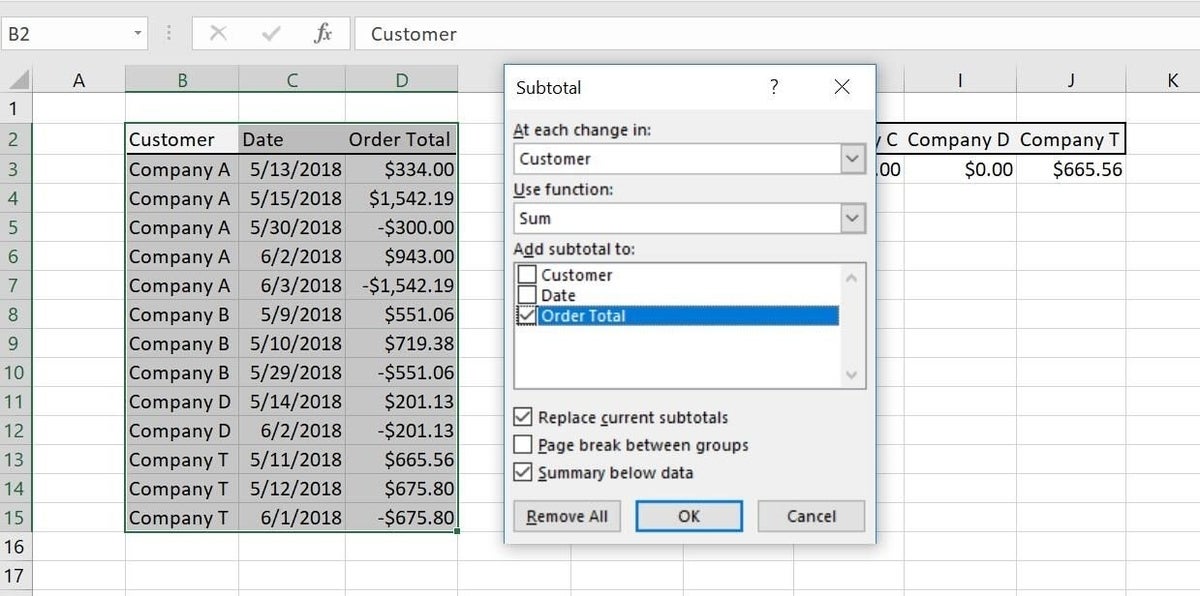
Excel’s Subtotal feature might be an option for summing. When using this feature, sorting the data is always the first step. In this case, we want to sum by customer, so you’d first sort by the Customer field. Then, click anywhere inside the data set and continue:
- Click the Data tab and then click Subtotal in the Outline group.
- In the resulting dialog, select Customer from the At each change in dropdown.
- Choose Sum from the Use function dropdown.
- Check Order Total in the Add subtotal to list (Figure E).
- Click OK to see the results shown in Figure F.
Figure E
Choose Subtotal settings.
Figure F
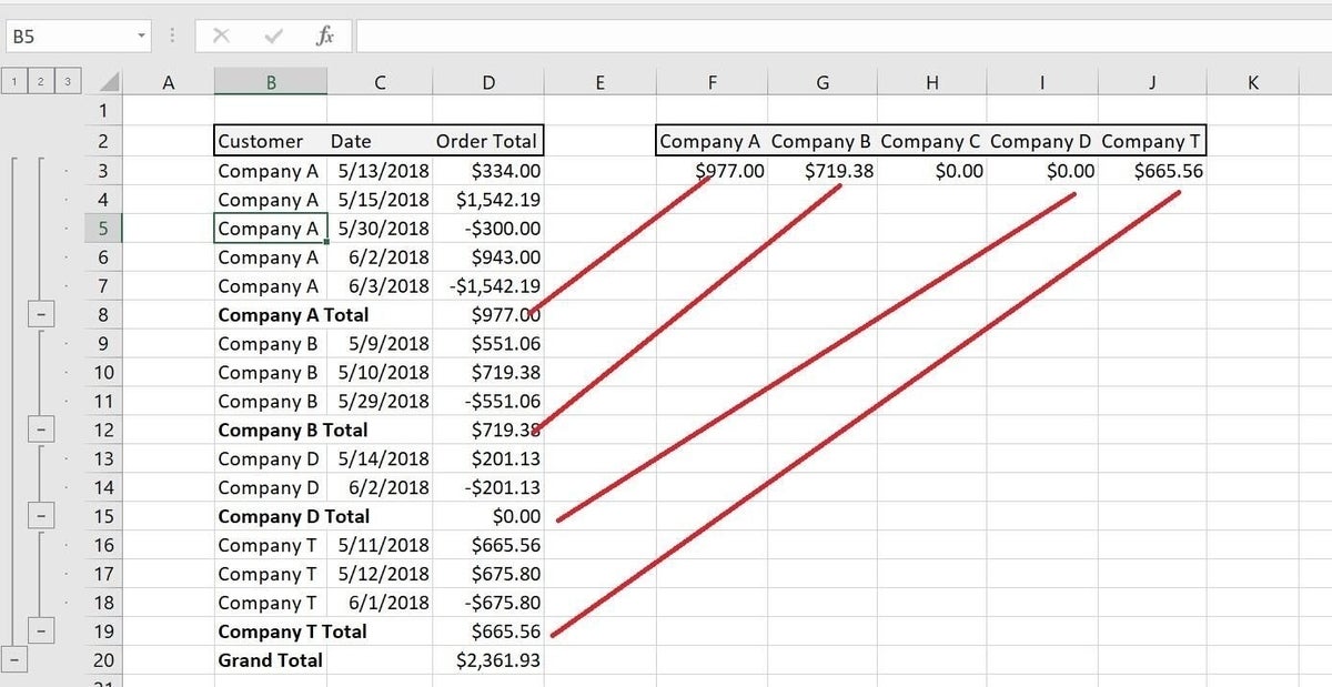
Subtotal returns the same results as the SUMIF() matrix.
The Subtotal feature returns the same results as the matrix but displays the relevant details with the subtotals. It’s not dynamic, however. Nor can you easily return subtotals for the Customer and Date data, at least, not as is. To accommodate both would require some initial setup and even then, it’s still not dynamic. Subtotal is a toggling feature and you can turn it off and on to update results as you add data.
PivotTable
Excel’s PivotTable feature probably offers the best choice. You don’t have to sort the data set first, you can filter by dates, and by basing the PivotTable on a Table object you refresh the PivotTable after updating the data set. First, let’s convert the data set into a Table as follows:
- Click anywhere inside the data set, click the Insert tab, and then click Table in the Tables group.
- In the resulting dialog, check the data range (it should be correct).
- Check the My table has headers option.
- Click OK.
Now you’re ready to create the PivotTable as follows:
- Click anywhere inside the Table.
- Click the Insert tab and click PivotTable in the Tables group.
- Click New Worksheet if necessary and click OK.
- Using the PivotTable Field pane, drag Customers to the Rows list and drag Order Total to the Values list.
- Next, drag Date to the Rows list. When you do, Excel will add a Months field, automatically. Drag Months from the Rows list to the Filters list (Figure G).
Figure G
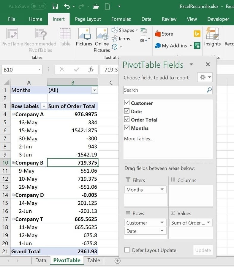
The PivotTable displays details, subtotals, and allows you to filter by the month.
At this point, you have detail records and subtotals grouped by company. You’re not matching payments to invoices, but you can see at a glance which companies have an outstanding balance. To filter subtotals by the month, use the filter. As you can see in Figure H, June’s details and totals show mostly payments. You can also filter by company by choosing an option from the Row Labels dropdown. (If your data set has distinct columns for debit and credit add those to the Rows list.)
Figure H
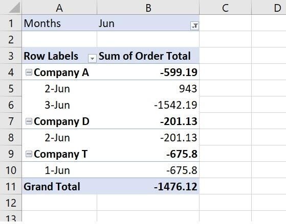
Use the filter to display records by the month.
The PivotTable will reflect changes to the Table, even new records. After updating the Table, click inside the PivotTable, click the Contextual Analyze tab and then click Refresh in the Data group.
Send me your question about Office
I answer readers’ questions when I can, but there’s no guarantee. Don’t send files unless requested; initial requests for help that arrive with attached files will be deleted unread. You can send screenshots of your data to help clarify your question. When contacting me, be as specific as possible. For example, “Please troubleshoot my workbook and fix what’s wrong” probably won’t get a response, but “Can you tell me why this formula isn’t returning the expected results?” might. Please mention the app and version that you’re using. I’m not reimbursed by TechRepublic for my time or expertise when helping readers, nor do I ask for a fee from readers I help. You can contact me at susansalesharkins@gmail.com.
Also see:
- How to create multilevel numbered headings in Word 2016 (TechRepublic)
- Office Q&A: How to use color to identify incoming Outlook messages (TechRepublic)
- 3 ways to display meaningful information in Excel using budget values (TechRepublic)
- 5 ways to delete blank rows in Excel (TechRepublic)
- How to combine and analyze data from multiple data sets using Excel Power Pivot (TechRepublic)