


An expression to return a simple running total in Excel is easy — a few references and you’re done. A conditional running total takes more work. The expressions aren’t difficult and don’t require a lot of specialized knowledge, but they can be more work than necessary, especially if you’re reporting the results. In this article, I’ll show you how to calculate a conditional running total using an Excel PivotTable without any expressions at all. Once you have a simple running total in a PivotTable, a conditional running total is a simple matter of grouping the right fields.
SEE: Software Installation Policy (TechRepublic)
More about Software
- Software Installation Policy
- Five Methods to Insert a Checkmark Into Microsoft Office Products
- How to Hide and Handle Zero Values in an Excel Chart
- How to Use Section Breaks to Control Formatting in Word
I’m using Microsoft 365 on a Windows 10 64-bit system, but you can use earlier versions of the .xlsx format through 2007. Excel for the web supports PivotTable objects. For your convenience, you can download the .xlsx demonstration file.
If you’re not familiar with PivotTable objects yet, consider reading How to use Excel’s PivotTable tool to turn data into meaningful information. If you’d like to learn how to generate a conditional running total at the sheet level, read How to calculate conditional running totals in an Excel revenue sheet.
What’s a running total?
A running total is similar to your checking account. Money goes in and money goes out, and each transaction contributes to the account’s balance, or in this case, the running total on any given day. Technically, a running total is a cumulative sum that includes previous transactions as well as the current, within a given period.
Excel expressions can be used to return a running total in an Excel sheet, but Excel’s PivotTable might be quicker than expressions because you don’t have to know the math—the PivotTable has a running total option.
The data
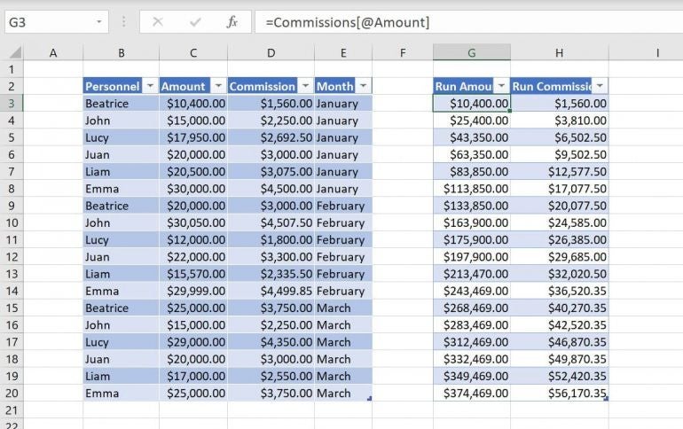
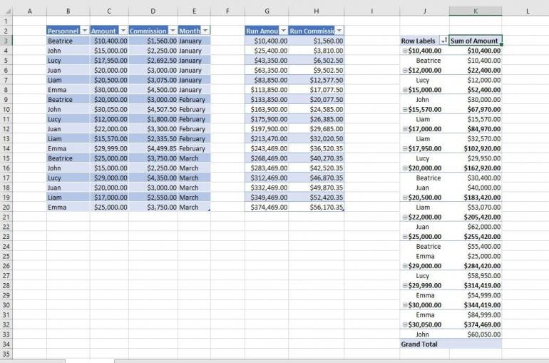
Figure A shows a simple sheet of commissions for six employees over a three-month period. The Table to the right shows a running total for the Amount and Commission columns. The sheet has two Table objects. The four-column Table is named Commission, and the two-column Table is named RunningTotals.
Figure A
The expressions in G3 and H3 are simple references to the first value in each column:
G3: = C3
H3: = D3
The running total expressions in G4 and H4 follow:
G4: =Commission[@Amount]+G3
H4 =Commission[@Commission]+H3
or
G4: =G4+G3
H4: =H4+H3
if you’re not using a Table object.
Then those expressions are copied to the remaining cells. The structured reference expressions and the simple references are the same—the only difference is the type of referencing—use the simple referencing if you’re not working in a Table object.
Now, let’s create a PivotTable.
How to create a PivotTable in Excel
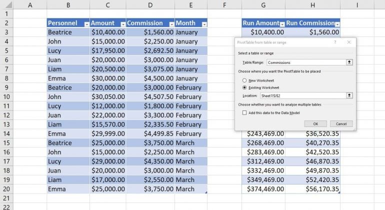
We’ll begin by building a simple PivotTable based on the Commission Table that displays the same results more or less as the RunningTotals Table shown in Figure A. To get started, click anywhere inside the Commission Table (four columns) and then do the following:
- Click the Insert tab and then click PivotTable in the Tables group.
- In the resulting dialog, click Existing Worksheet, so you can see the data and the PivotTable.
- Click inside the Location control and then click J2 in the sheet (Figure B).
Figure B
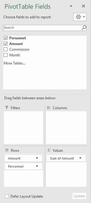
- Click OK. At first, the PivotTable is blank.
- Click the frame to display the PivotTable Fields pane. If it doesn’t appear, right-click the frame and choose it from the resulting dialog.
- Using Figure C as a guide, drag fields to the lists below.
Figure C
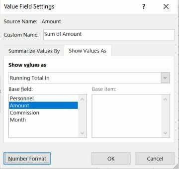
- Right-click any cell in the Sum of Amount column and choose Value Field Settings from the resulting submenu.
- Click the Show Values As tab and select Running Total in from the Show Values As dropdown.
- Make Sure Amount is selected in the Base Field list (Figure D).
Figure D
- Click the Number Format button and select Currency from the Category list.
- Click OK twice to return to the PivotTable shown in Figure E.
Figure E
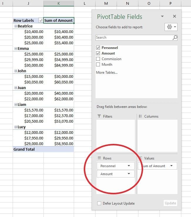
You could create a PivotTable for Commission by replacing the Amount fields with the Commission fields in the PivotTable Fields pane. As is, it’s hard to determine how Excel sorted the names and amounts. Note the order of the fields in the Rows list (in the PivotTable Fields pane). This will come up again later. Their positions matter when grouping.
If you start moving fields around, the PivotTable starts grouping, which is what we want to see next.
How to make a conditional running total in Excel
At this point, you’ve not really gained much; the PivotTable isn’t really any better than the Table and its simple expressions. The difficulty comes in when you want conditional running totals. For instance, an expression that returns a running total for each person instead of the full column of values, takes a bit of know-how. On the other hand, the PivotTable requires only a bit of rearranging.
SEE: Why Microsoft Lists is the new Excel (TechRepublic)
First, Figure F shows the result of rearranging the two fields in the Rows list. Simply click one and drag it above or below the other. Not only does the PivotTable return a running total for each person, but it also sorts the groups in a meaningful way.
Figure F
Now let’s suppose that you want a running total for each month and the personnel isn’t relevant. In the PivotTable Fields pane drag personnel back up to the fields list. Then, drag Month down, positioning it above Amount, as shown in Figure G.
Figure G
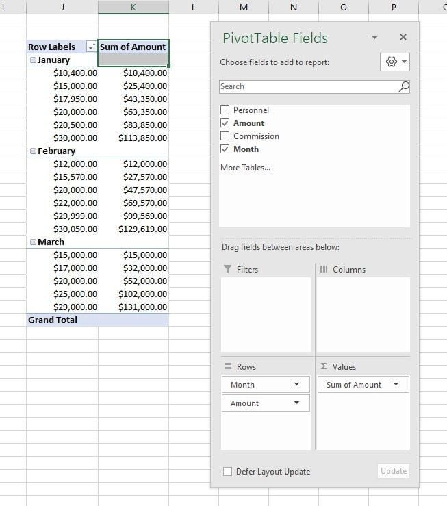
Moving a few fields around in the PivotTable Fields list is much easier than coming up with a conditional expression for the sheet level. If you know how to create a simple running total in a PivotTable, conditional running totals is only a click away!